This time is different. –John Templeton
“This time is different,” is a sentiment that leads many investors to stray from using data analysis in their investment decision process and more towards discretionary judgment. The logic as to why data analysis techniques may not apply to “different” situations is often framed in the following way:
These particular set of conditions have never occurred before, therefore no historical data points are relevant to verify my strategy.
This opinion is technically true. The market on a given day is not exactly like any historical data point. If an investor’s viewpoint is that previous data points are only valid if collected in identical conditions as the present scenario, then that investor cannot use historical data to validate (or invalidate) their trade hypothesis.
But herein lies the problem: market conditions are always unique. Let’s go to the absolute extreme so we can see that even in an unrealistic scenario, we would still see different market conditions.
In this theoretical situation, there are two straight days where there are no earnings reports and no financial metrics that are released. There is no news globally that is significant in any sector that could remotely impact the markets. Even the behavior of the market itself is identical from day 1 to day 2. Similarly, all asset classes have identical behavior from day 1 to day 2. We can say the market volume is also steady from day 1 to day 2.
It doesn’t matter what the market movement is; it can stay the same, it can drop, it can rise. When faced with the question, “Are the market conditions identical to what there were prior to day 1?”, the answer is “no.” It matters that the market has behaved in a particular way for two days, as opposed to one day. The very sequence of events creates a unique scenario, even if all other variables have remained constant.
This example is meant to demonstrate a simple lesson: if we cannot use data analysis when a situation is “unique”, as it disqualifies all historical data points, then we can never use data analysis, as a situation is always “unique.”
Below is a sample performance of a strategy that has three distinct stages: the period prior to utilization of the strategy, with which its performance justified its usage, the first stage in which the strategy performed well, and the most recent stage in which the performance has been poor, which ends in the present. In the backgrounds of the performance are “x” and “-“ symbols, which represent market conditions that are present at the time.
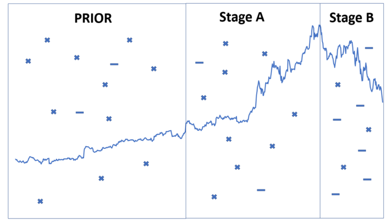
Viewing this chart qualitatively leaves it wide open to interpretation. With the benefit of hindsight, an investor can deduce multiple reasons as to why their strategy is not working in Stage B. “This works best when there is a higher concentration of ‘x’, as it was prior and in Stage A.” This is clear from the chart above to true. Similarly, “the strategy doesn’t perform as well when the amount of ‘-‘ is present, so I should take the strategy off now”, is also a reasonable statement.
However, as we saw previously, market conditions will never be identical from one period to another. There will always be differences in market conditions, and an investor can always point to those as being a reason to activate and deactivate a strategy.
Does this mean that we should just ignore market conditions, as the only constant is that they are always changing? Of course not. We can employ a specific strategy to help quantify these conditions and be systematic in the manner in which we analyze our data to account for the shift in conditions.
How can we use historical data points if they do not occur in identical conditions as the current market? The easy answer is to disregard the conditions, and accept that the conditions will always be different. A difficult but more responsible approach would be to develop general quantifiable conditions from which we can gather relevant historical data points.
Let’s look at those two characteristics one at a time. The conditions should be general because if they are too specific the sample size will be too small to develop confident conclusions. This is the constant balance that data scientists must deal with. The more relevant the data points you seek to find, the fewer of them there will be, and thus the less confidence that can be gained from historical patterns. The less relevant the data points, the larger the sample, but the less predictive those data points are likely to be, as many will have occurred in conditions that are less of a reflection of the present situation.
When choosing how general the conditions are to be when considering the evaluation of a particular investment strategy, it may help to start more general, and get more specific until you’ve reached a point where the number of data points is prohibitively small.
Now for the second characteristic: your conditions must be quantifiable. How you choose to quantify those conditions may be somewhat arbitrary, but by choosing an objective measure to delineate one condition from another enables you to back-test efficiently. For example, you may have a strategy that you want to use during “bull markets.” There are a variety of ways you can choose to quantify market movements so you can categorize the conditions as being a ‘bull’ market or a ‘bear’ market. You can say that if the 5-day simple moving average moves below the 50-day simple moving average, it’s no longer a ‘bull’ market. Armed with that metric, you can objectively determine your ‘bull’ or ‘bear’ designation going back decades so you can apply strategy and back-test its performance.
Below is the same chart we saw above, this time with the 5-day and 50-day simple moving averages charted:
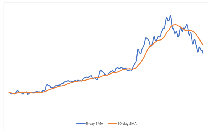
Because we now have quantified the indicator we are looking at (5-day vs 50-day SMA), we can objectively determine whether these conditions justify turning off the strategy. Instead of looking at average gains and losses, we will simplify a bit and just view whether or not the day after our 5-day vs 50-day SMA reading was profitable or unprofitable. Using the data from the “Prior” and “Stage A” only yields the table:
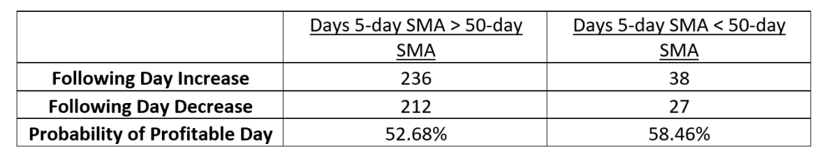
How strange! It turns out that if the 5-day SMA was below the 50-day SMA, suggesting negative momentum, the following day was MORE likely to be profitable, than if the 5-day SMA was above the 50-day. Without this analysis, it would be easy to look at the performance in “Stage B”, determine that more losses are incurred when the 5-day SMA is below the 50-day SMA, and wait until the condition has shifted.
This analysis also demonstrates how powerful quantifying conditions can be versus using the naked eye. If you asked 10-people if the strategy was more likely to profitable if the blue line was above or below the orange line in “Prior” and “Stage A”, most would probably give the incorrect response. Quantifying these conditions protects ourselves from making emotional decisions and exposing our hypotheses to experiential and recency biases.
You can read an excellent article here on taking a Bayesian approach to evaluating your existing investing strategy. To summarize, when you first chose your investment strategy, it was likely not done so at random. There must have been historical data that supported the trade hypothesis, otherwise the strategy would not be pursued. Even if the strategy does not perform up to standards in the short term, the Bayesian approach takes the performance PRIOR to utilizing the strategy into account. This prevents too much weight from being placed on a small sample size, which tends to scare off many investors.
A typical response to this thinking may be that the strategy was designed for a different market environment, and now “things have changed.” This is precisely why specific market conditions must be quantified AHEAD of time, such that when those conditions DO change, the efficacy of the strategy in those conditions has already been validated.
Let’s look at two examples, one in which the investor anticipates specific conditions and quantifies the impact of those conditions on their strategy, and one in which they do not.
First, let’s assume the investor neglects to foresee a change in conditions. After reviewing historical data, the investor believes a particular strategy will generate significant alpha over time. They activate the strategy, and 6 months into trading, the macro-market shifts from a bull market into a bear market, and the strategy has a negative alpha during the testing period.
Using the Bayesian approach, the investor finds they can still have a high confidence in the strategy, as the historical data prior to actively trading carries more weight than the previous 6 months, so even though their confidence may be slightly less after the recent setbacks, their strategy is still quantitatively solid.
However, the investor talks themselves into discounting that historical data. “That was a different market,” they say, downplaying the strong performance their strategy had prior to trading it actively, “this strategy would have been a loser if the market before was in the same state that it is today.” They take the strategy off, believing the timing is no longer ripe.
Now, let’s look at the investor who anticipates a shift in conditions. Not only do they find the historical data to be strong, but they quantify the confidence they have in their strategy in a variety of different quantifiable conditions. They categorize different historical markets as being “bull” or “bear” markets, and even look at periods where specific outside factors may impact the market, such as news related events (like elections) and the behavior of other asset classes. Armed with confidence levels for various categorical markets, the investor begins trading the strategy.
6 months in, the market turns from a bull into a bear. This isn’t a subjective measure; abiding by the methodology they employed when reviewing the historical data, the investor can say specifically how their system categorizes the present market state. Based on that market state, the investor can view the confidence level of their strategy in that market, and make a decision.
Whether the investor decides to pull the investment off or not is irrelevant at this point. Their decision will be based on a quantifiable confidence specific to the present market conditions. Will the conditions used in the historical data as an analog to the present market be perfect? Of course not. But it will reflect the general behavior at this point in time enough such that the investor will be taking the underlying mood of the market into account in a quantifiable way.
Front-loading the analysis will make your life easier when it comes time to make decisions when everyone else is being emotional. You will have already made your decision prior to the actual shift in the market because you had tested your strategy against different conditions. This saves you lots of time, and equally importantly, will empower you to make an objective, disciplined decision instead of acting out of fear.(1)

References[+]
| ↑1 | See here for a piece on ‘Trying Too Hard' |
|---|
About the Author: David Primer
—
Important Disclosures
For informational and educational purposes only and should not be construed as specific investment, accounting, legal, or tax advice. Certain information is deemed to be reliable, but its accuracy and completeness cannot be guaranteed. Third party information may become outdated or otherwise superseded without notice. Neither the Securities and Exchange Commission (SEC) nor any other federal or state agency has approved, determined the accuracy, or confirmed the adequacy of this article.
The views and opinions expressed herein are those of the author and do not necessarily reflect the views of Alpha Architect, its affiliates or its employees. Our full disclosures are available here. Definitions of common statistics used in our analysis are available here (towards the bottom).
Join thousands of other readers and subscribe to our blog.