A new DFA article by Rizova and Saito (2019, “Investment and Expected Stock Returns”) (1) rehashes previous arguments in Fama and French (2006, 2015) on the investment factor.
The core arguments are as follows:
- Valuation theory predicts that expected investment is negatively correlated with expected return, all else equal; and
- Current asset growth is a good proxy for expected investment.
According to Fama and French, the negative relation between expected investment and expected return gives rise to the investment factor, which captures the negative relation between current investment and expected return in the data.
In this blog, which is broken into 5 sections, I show that Fama and French’s arguments are fundamentally flawed (Hou et al. 2019a). I also describe the conceptual foundation of the investment factor in Hou, Xue, and Zhang (2015), a foundation which, in my view, better reflects the underlying economics of the investment factor.(2)
1. A Positive Relationship between Expected Investment and Expected Return in Valuation Theory
In Fama and French’s formulation of valuation theory, the discount rate is the internal rate of return, which is constant over time. While a useful concept, the constant discount rate return clearly contradicts the well-accepted notion of time-varying expected returns. For instance, it is nowadays well accepted that expected returns are higher in recessions than in booms, due to higher risks, higher risk aversions, or more investor pessimism in recessions.
Hou et al. (2019a) reformulate valuation theory with a one-period-ahead expected return. They show that the relation between expected investment and the one-period-ahead expected return is more likely to be positive in the reformulated valuation theory. In addition, the same relation is also positive in the investment CAPM, which is the conceptual foundation of the q-factor model (see Section 3 below).
Empirically, Fama and French (2006) in fact report a positive, albeit weak, relation between expected investment and expected return. They write:
“Contrary to the predictions of the valuation equation (3), however, the return regressions of Table 3 produce positive average slopes on the Table 2 regression proxies for expected asset growth, but they are not reliably different from zero.” Fama, Eugene F., and Kenneth R. French, 2006, Profitability, investment and average returns, Journal of Financial Economics 82, 507.
Specifically, in Table 3 reproduced below, the highlighted column is the slopes on expected investment in monthly cross-sectional return regressions. The slopes are mostly positive, albeit insignificant. The evidence says that expected investment estimated via their specifications is positively related to the expected return, although the relationship is weak.
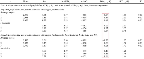
Table 3 in Fama and French (2006): Monthly cross-sectional return regressions The results are hypothetical results and are NOT an indicator of future results and do NOT represent returns that any investor actually attained. Indexes are unmanaged, do not reflect management or trading fees, and one cannot invest directly in an index.
2. Current Asset Growth Is a Poor Proxy for Expected Investment
Continuing on the path of a negative relation between expected investment and expected return, Fama and French (2015) ditch the two specifications of expected investment in Table 2 of their 2006 article and switch to current asset growth as the proxy for expected investment. Doing so yields a desired negative relation between expected investment and expected return. However, current asset growth is a poor proxy for expected investment.
The evidence is borne out in Table 2 in Fama and French (2006) reproduced below. The table shows annual cross-sectional regressions of future asset growth on lagged firm variables, one of which is current asset growth. If asset growth is a perfect proxy for expected asset growth, the slopes on current asset growth should be close to one and drive out all other variables. However, the first highlighted column below does not support this view. In the shorter specification, the slopes on asset growth are economically small, albeit significant, indicating weakly positive autocorrelations of asset growth. In the longer specification, the slopes on asset growth are all virtually zero and insignificant.
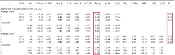
Table 2 in Fama and French (2006): Multiple regressions to predict asset growth The results are hypothetical results and are NOT an indicator of future results and do NOT represent returns that any investor actually attained. Indexes are unmanaged, do not reflect management or trading fees, and one cannot invest directly in an index.
Further evidence is provided in Table VII in Hou et al. (2019a) reproduced below. The table shows annual cross-sectional regressions of book equity growth on current asset growth and, separately, on current book equity growth. The first highlighted column shows that the slopes on current investment when predicting future investment are far from one, 0.2 in the first year and quickly falls afterward. The R-square starts at 6% in year one and falls largely to zero afterward.
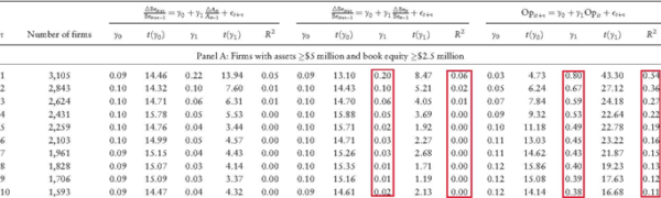
Table VII in Hou et al. (2019a): Annual cross-sectional regressions of future book equity growth and future operating profitability The results are hypothetical results and are NOT an indicator of future results and do NOT represent returns that any investor actually attained. Indexes are unmanaged, do not reflect management or trading fees, and one cannot invest directly in an index.
The last five columns in the table show the cross-sectional regressions of operating profitability on current operating profitability. Operating profitability is substantially more persistent than investment, the slope in the first year is 0.8, and the R-square 0.54. This evidence supports Fama and French’s (2015) use of operating profitability as expected operating profitability in their 5- and 6-factor models as well as Hou, Xue, and Zhang’s (2015) use of current return on equity (Roe) as expected Roe in the q-factor model.
In sum, the evidence is clear that current asset growth is a poor proxy for expected asset growth, but current operating profitability is a good proxy for expected operating profitability. The evidence casts doubt on Fama and French’s (2015) arguments of the investment factor via the expected investment channel.
3. Investment, Expected Investment, and Expected Stock Returns: The Investment CAPM Perspective
In the investment CAPM (Zhang 2017), investment and expected investment are related to expected return in two different ways.
In particular, Hou, Xue, and Zhang (2015) propose the investment factor as a key driving force of expected stock returns. In Corporate Finance, the net present value (NPV) of a project is its present value (discounted value of the project’s future cash flows) minus its investment costs today. The NPV rule says that a manager should invest in a given project, if and only if the present value of the project is greater than or equal to its investment costs.
When initially facing many projects with nonnegative NPVs, the manager should start with the project with the highest NPV and work her way down the supply curve of projects. A good project has a low discount rate, high profitability, and low investment costs. As the manager takes more and more projects, their investment costs become higher and higher, and their profitability lower and lower. For the last project that the manager takes, its NPV should equal zero:
- (A) Investment costs = Present value = Profitability/Discount rate.
The investment CAPM turns the NPV rule, which is a fundamental principle in Corporate Finance, on its head and transforms it into an Asset Pricing theory. Rewriting the NPV rule yields:
- (B) Discount rate = Profitability/Investment costs.
Relative to profitability, high investment firms incur higher investment costs, meaning that their discount rates and expected returns must be low. Relative to investment, high profitability firms must have high discount rates and high expected returns. In all, investment and profitability are two key driving forces of expected stock returns.
The investment factor arises naturally from equation (B). Intuitively, given profitability, high costs of capital (discount rates) imply low NPVs of new projects and low investments, and low costs of capital imply high NPVs of new projects and high investments.
Equations (A) and (B) apply to a static model with only one period. In a multiperiod, dynamic model, equation (A) becomes:
- (A) Investment costs = Present value = (Profitability + Present value of cash flows from next period onward)/Discount rate.
However, with optimal investment, the present value of cash flows from the next period onward equals expected investment costs next period (marginal q equals marginal costs of investment). Accordingly, equation (B) becomes:
- (B) Discount rate = (Profitability + Expected investment costs)/Investment costs.
Intuitively, if investment and expected investment costs are high next period, the present value of cash flows from the next period onward must be high. Because the benefits to investment this period are primarily the present value from the next period onward, the benefits to investment this period must also be high. As such, if expected investment costs are high next period relative to investment costs this period, or equivalently, if the expected investment is high next period relative to current investment, the discount rate must be high. The discount rate must be high to offset the high benefits of investment in this period to keep the current investment low.
This intuition behind the positive relation between expected investment (growth) and expected return is analogous to the intuition behind the positive relation between profitability and expected return, i.e., the Roe factor in the q-factor model. And this is the core intuition underlying the expected investment growth factor in the model of Hou et al. (2019b).
4. Factor Spanning Tests: The q-factor model versus the Fama-French (2018) 6-factor model
The discussion so far has been largely conceptual. To get a sense of empirical performance, the following table updates the factor spanning tests in Hou et al. (2019a). The tests show that the q-factor model cleanly subsumes the Fama-French 6-factor model in head-to-head contests.
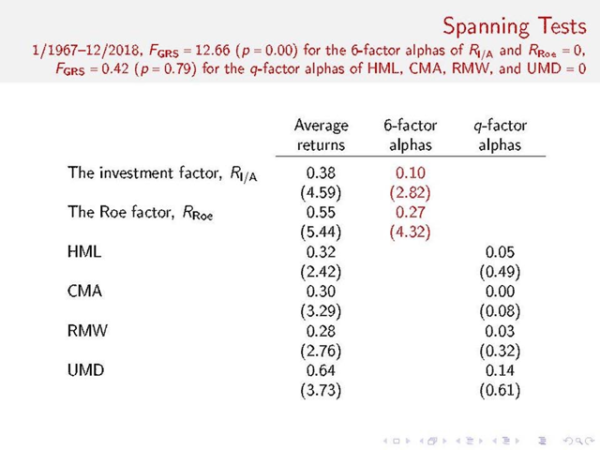
Specifically, in the 1967-2018 monthly sample, the investment and return on equity (Roe) factors in the q-factor model earn on average 0.38% and 0.55% per month (t = 4.59 and 5.44), respectively. Their alphas in the Fama-French 6-factor regressions are 0.1% and 0.27%, both of which are significant (t = 2.82 and 4.32), respectively. The Gibbons, Ross, and Shanken (GRS, 1989) test strongly rejects the null hypothesis that the Fama-French 6-factor model can subsume the investment and Roe factors. In all, despite having two more factors, the Fama-French 6-factor model cannot subsume the q-factor model in the data.
Conversely, HML, CMA, RMW, and UMD in the Fama-French 6-factor model earn on average 0.32%, 0.3%, 0.28%, and 0.64% per month (t = 2.42, 3.29, 2.76, and 3.73), respectively. More important, their alphas in the q-factor regressions are economically small (tiny in many cases) and statistically insignificant: 0.05%, 0.00%, 0.03%, and 0.14% (t = 0.49, 0.08, 0.32, and 0.61), respectively. The GRS test cannot reject the null hypothesis that the q-factor model can subsume the HML, CMA, RMW, and UMD factors. In all, despite having two fewer factors, the q-factor model fully subsumes the Fama-French 6-factor model.
5. Summary
This blog shows that Fama and French’s (2006, 2015) arguments for the investment factor are fundamentally flawed. Valuation theory, once reformulated in terms of the one-period-ahead expected return, implies a positive relation between expected investment and expected return, a positive relation which Fama and French’s (2006) own evidence supports. In addition, unlike profitability, firm-level asset growth is not persistent, meaning that current asset growth is a poor proxy for expected investment.
The investment factor arises more naturally from the investment CAPM, which in essence is a restatement of the Net Present Value rule in Corporate Finance. Intuitively, given profitability, high costs of capital (discount rates) imply low NPVs of new projects and low investments, and low costs of capital imply high NPVs of new projects and high investments.
Finally, empirically, factor spanning tests show that the q-factor model cleanly subsumes the Fama-French (2018) 6-factor model in head-to-head contests.
References
Fama, Eugene F., and Kenneth R. French, 2006, Profitability, investment and average returns, Journal of Financial Economics 82, 491-518.
Fama, Eugene F., and Kenneth R. French, 2015, A five-factor asset pricing model, Journal of Financial Economics 116, 1-22.
Fama, Eugene F., and Kenneth R. French, 2018, Choosing factors, Journal of Financial Economics 128, 234-252.
Hou, Kewei, Haitao Mo, Chen Xue, and Lu Zhang, 2019a, Which factors? Review of Finance 23, 1-35.
Hou, Kewei, Haitao Mo, Chen Xue, and Lu Zhang, 2019b, , working paper, The Ohio State University.
Hou, Kewei, Chen Xue, and Lu Zhang, 2015, Digesting anomalies: An investment approach, Review of Financial Studies 28, 650-705.
Rizova, Savina, and Namiko Saito, 2019, Investment and expected stock returns, Dimensional Fund Advisors.
Zhang, Lu, 2017, The investment CAPM, European Financial Management 23, 545-603.

About the Author: Lu Zhang
—
Important Disclosures
For informational and educational purposes only and should not be construed as specific investment, accounting, legal, or tax advice. Certain information is deemed to be reliable, but its accuracy and completeness cannot be guaranteed. Third party information may become outdated or otherwise superseded without notice. Neither the Securities and Exchange Commission (SEC) nor any other federal or state agency has approved, determined the accuracy, or confirmed the adequacy of this article.
The views and opinions expressed herein are those of the author and do not necessarily reflect the views of Alpha Architect, its affiliates or its employees. Our full disclosures are available here. Definitions of common statistics used in our analysis are available here (towards the bottom).
Join thousands of other readers and subscribe to our blog.