Introduction
This project builds on research conducted by J. Piotroski, who published his paper Value Investing: The Use of Historical Financial Statement Information to Separate Winners from Losers in 2000, offering a simple yet powerful framework to separate the winners from the losers in a value-investing context (summary here). You can read about how Piotroski’s research is utilized as a quality screen by our firm here (and a piece on improving Piotroski here by Alpha Architect).
Several things differentiate this project from the original work by Prof. Piotroski:
- New factors. Since the time of the original publication, the investment industry has witnessed a proliferation of anomalies, or factors, with new ones being discovered every year. Some anomalies even made it into a new, five-factor Fama & French model(1). I have reviewed all the major papers published between 2000 and 2018 and collected most of the factors related to accounting variables as well as certain market variables and tested them in a joint framework to find out which of them actually work.
- A novel approach to factor construction. Several of the factors are constructed using a less-known method called “Q-scoring”. I elaborate on this approach further in this paper.
- A stricter, more balanced definition of “undervalued”. In his paper, Prof. Piotroski separates all public stocks into quintiles according to their B/M values and takes the highest quintile (with the highest B/M). For reasons outlined in this paper, I sort the companies according to the ratio of their book value of invested capital to the market value of invested capital (BVIC/MVIC). I also neutralize this metric so that it is not artificially tilted toward certain countries and industries that are cheap on average, given that this cheapness may be dictated by the fact that the market is pricing in some systemic macro risk, rather than that the companies belonging to these countries or industries are undervalued.
- Applying a method from the field of forensic accounting. I download all the financial statements items for each company and calculate a so-called “Benford score”, which is a wholly uncorrelated factor that is able to detect financial statement fraud using only mathematics. Further detail will be given below.
- A guided search for significant factors. Unlike Prof. Piotroski, who allegedly came up with his nine signals through studying professional and academic articles, picking the ones suited to his professional taste and acumen, I employ an algorithm similar to a machine learning method called boosting(2) to find the best-performing set of variables.
Initial Universe Screen
I test my strategy for returns relating to years 2007-2018. Data(3) is downloaded for years 2005-2018 (since some variables require at least two years of data). Because the strategy is fundamentals-based and requires fiscal year-end reports, the screening procedure consists of sifting all public listed stocks through criteria that are effective as of April, 30th, each year, since this is when most companies will have published their fiscal year-end reports.
Here are the main criteria for the screen:
- Company type: Public, active, listed companies
- Security type: Common stock
- Market cap as of April, 30th: >$50 million
- Excluding Financials (since for this sector classical financial ratios are widely considered less applicable)
Addressing Various Backtesting Biases
Overfitting. To eliminate overfitting, the data set is separated into a training set and a testing data set. The model is trained on the years 2007-2016 and tested on 2017-2018. To ensure that the results are not spurious, the model is finally tested on a subset of both the training and the testing data sets that represent European companies only(4)
Look-ahead bias. This is a fairly common mistake of backtesting procedures, since most researchers lack sophisticated analytical proprietary databases that are able to download only data that has been available starting a certain “as of” date. Luckily, the Capital IQ database lets the researcher do exactly this. Consequently, one can be sure that the fundamentals that are downloaded as of each April 30th were readily available on that date.
Issues with market capitalization and liquidity. A minimum floor of a $50 million Market cap is one of the things that ensures that the strategy is practically implementable since it eliminates micro-caps that are very thinly traded and have potential problems with liquidity, imposing high ex-ante returns that are actually very hard to harvest by a practitioner. This floor is used, in particular, by J. Greenblatt, the author of the widely acclaimed “magic formula investing”.
Survivorship bias. This bias is implicitly addressed by the possibility of the Capital IQ database to screen for companies that had certain characteristics at a certain time.
Insufficient sample bias. The joined training data set contains 14,565 companies and spans 10 years, with two more years for out-of-sample testing. This includes all the companies with the above-mentioned characteristics that existed during the years 2005-2017 and had those characteristics on April 30th of any given year. The smallest year-sample is for 2005, listing 3617 companies. This is more than enough for any statistically meaningful inferences in regard to the effectiveness of a particular strategy.
Data-mining bias. Firstly, this is addressed by the fact that all variables that I used were taken from academic literature or inspired by it, ensuring that they all have a sound economic basis for them. Secondly, instead of a blind searching process that tests all possible combinations(5), I set up a logical process of step-by-step addition of factors where each next factor addresses the shortfalls of the previous ones. Overall, I identify eight significant factors that prove to be the most beneficial in terms of implementation of a strategy, which is one factor less than was identified by Piotroski, further reducing the probability that the results can be somehow attributed to pure chance.
Value Factor Screen
In his initial work, Prof. Piotroski tested whether a financial analysis-based strategy can improve upon a simple strategy of buying value stocks(6). He used a widely known value metric B/M, which is the relation of equity book value to its market value. This metric does not take into account three important things:
First, the B/M ratio disregards the effects of financial leverage on companies’ attractiveness. Consider two similar companies; each has a B/M of 1.5 (a hypothetical situation that assumes both companies are trading at roughly 0.67 times the book value of their equity). To bring this number to life, let us assume that both companies have $150m of equity on their books and their capitalizations are $100m. For a hypothetical value investor who judges by the B/M metric alone, it would seem like a bargain and she would be indifferent as to which of the companies to buy. However, company A has $200m of debt on its balance while company B has zero leverage. While the reader may have already guessed that given the limited information, it would be more prudent to choose company B since it is probably less distressed, there is a way to show this mathematically. We calculate for both companies BVIC/MVIC, the ratio of book value of invested capital to its market value(7). Company A’s BVIC/MVIC is (150+200)/(100+200)=1.17, whereas Company B’s ratio is still 1.5. Ben Graham would say that Company B has a wider “margin of safety” in terms of its firm value, i.e. its assets are trading at a steeper discount.
Second, the B/M ratio disregards the fact that during certain periods of time, various industries and countries may be “cheap”, i.e., have high average B/M multiples for reasons other than undervaluation. For example, consider an economic crisis in a certain country. Alternatively, a sudden technological shift that prompts capital outflows from an industry. These events may cause such industries or countries to take up disproportionately high weights in a portfolio sorted on a purely B/M basis. This is why, having computed the BVIC/MVIC for each company, I neutralize each ratio through the following arithmetic adjustment:

Third, book value of equity is frequently a negative number, and this distorts the meaning and interpretability of the B/M ratio. The proposed BVIC/MVIC lacks this disadvantage since the sum of all invested capital is by definition a positive number.
I test the strategy on the top tercile(8) of companies according to their Adjusted BVIC/MVIC.
Types of Value Investing Variables Tested
I tested 73 variables in total. Most of them were handpicked from academic literature and represent certain fundamentals-based financial ratios. Some variables were calculated by me. All the variables were transformed into binary form in line with Piotroski’s work. All the variables I tested can be classified into roughly three major groups:
- Variables related to their own states in the past (horizontal analysis). This category includes things like “increasing margins” or “decreasing leverage”, which would be encoded as ‘1’ if true and ‘0’ otherwise. These variables require at least three years of firm data to be tested.
- Variables related to the medians (9) across their respective industry. These variables were first applied in a Piotroski-type framework by Partha S. Mohanram(10) who successfully showed that Piotroski’s general mode of thinking could be applied to “glamour”, or low B/M stocks to sift for winners among such stocks. This category includes such variables as “margins are higher than the industry median”, or “leverage is lower than the industry median”.
- Variables that cannot be classified into the above categories. This is the most interesting category. Financial theory tells us that many ratios have optimal levels that usually relate to their industry medians. These ratios do not easily fall into the logic “the higher (lower) – the better (worse)”, being more of the type that can be visualized in the form of a bell curve with the top point corresponding to some optimum state.
For example, one could reasonably assume that there is an optimal level of asset turnover (the relation of Sales to Assets) for a manufacturing firm. Too low a ratio would signal that the firm is under-utilizing its asset base. On the other hand, too high a ratio for a particular year may signal two things:
The firm is really good at utilizing its asset base, OR the firm is engaged in aggressive revenue recognition that will lead to underperformance in the near future (e.g. when the time comes to collect accounts receivable that turn out to be bad debt)
As another example, take a firm that works in distributions. If one looks at the levels of Inventory measured in relation to Sales, one can conclude that too high inventory levels are an (unnecessary) cost and could be indicative of excess stockpiling on the shelves. Too low Inventory levels, however, present a risk to the business since such a firm will have trouble managing an unexpected surge in demand and will consequently lose customers.
Such cases are usually resolved by a thorough financial analysis that looks into a particular firm’s past and present practices, considers abnormal balance sheet movements, and reads all the notes to the accounts. However, since I was looking for an implementable and (ideally) automated system of picking stocks, I needed a way to encode such an analysis into numerical form, preferably consisting of zeroes and ones.
This has set me thinking. For these types of ratios, I needed an indicator that would reward a firm’s closeness to the optimum. However, dynamics are important too – so I also needed an indicator that would reward the firm for progressing towards the optimum and penalize it for straying further from it.
I found the answer in the work of Stephen Penman(11) in the form of a measure called Q-score.
Although used for somewhat different purposes (namely, estimating the reasonableness of a firm’s policy towards building accounting reserves as an indicator of its earnings quality), it proved to be the ideal candidate.
To illustrate, let us assume that we would like to understand whether the firm has a reasonable level of Inventory-to-Sales and whether (if it is significantly different from the industry median) it is at least headed in the right direction.
The Q-score is a combination of two measures that respectively address both parts of this question.
The first measure, Qa, answers the question “How far away is the metric from the industry median?”, and is calculated as:

- The second measure, Qb, answers the question “How has the metric changed within the past year?”, and equals:

- The final measure, Q, is the simple average of the two:

- The closer it is to zero, the better. The logic of this indicator is best illustrated in the following matrix:
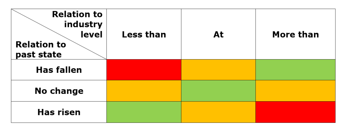
The green areas signify those states that should cause the least concern. The central piece captures the situation when the ratio is stable (there has been no change) and stays at or close to the optimum level. The bottom left piece considers the situation when the ratio has risen, but since the ratio is below optimal levels, this is a good situation. The piece on the upper right is the direct opposite, good as well.
Orange areas are areas of concern. They either capture situations when there is no improvement (when there should be) or when there has been a movement that led to the ratio coming close to the optimal level but since this movement may well continue into the future (a fair assumption, all else equal), it may pass the optimum mark into less optimal values.
Red areas are red flags. They signify that the ratio is both far from being optimal and is headed in the wrong direction.
Once the Q-score for each firm is computed, for each year, I sort them from largest to smallest and separate them into quartiles(12) using =QUARTILE(). The rule is that the 1st and the 4th quartile, corresponding to extremely positive or negative values (red zones in the above table), are encoded as zeroes, while the 2nd and the 3rd quartiles, corresponding to numbers that are closer to the optimum levels, are encoded as ones.
Final Value Investing Variables
Using a guided search procedure briefly described in the outline, I separated a subset of variables that conforms to the following criteria:
- Maximizing the percentage of winners in the portfolio (defined as companies that show positive returns). This criterion ensures that the returns are not driven by a few outperformers, by forcing the whole distribution of returns in a portfolio to be left-skewed (i.e., the bulk of returns are positive).
- Maximizing mean returns in a portfolio. These are returns produced by buying an equal-weighted portfolio of all the companies selected by the strategy.
The process is as follows. The first variable is selected that maximizes the combination of the above criteria if one were to select companies from the universe of undervalued stocks based solely on this variable. The variable should work across the whole training set, i.e. for the years 2007-2016.
The weights for each year are then readjusted based on the results of the initial variable chosen. Only then do they become the basis of a search for a new variable. The next variable should optimize ex-ante returns for the training set, given the new weightings. In practice, this means that the next variable is “judged” by how it deals with the years in which the previous variable was weak according to our criteria. The logic of this procedure is similar to a statistical method known as boosting. The process of adding on variables continues until the number of companies chosen by the model for each year reaches a reasonable count for a diversified portfolio (30-50 companies).
Eight variables made it into the final model:
- Increase in (cash and equivalents / current liabilities). This variable indicates that the situation with liquidity is improving in terms of the company’s ability to pay off its current liabilities with immediately available cash.
- Decreases in Current Assets. This variable might seem to be at odds with the previous one since Cash is part of Current Assets. However, coupled with the previous variable, it ensures that non-cash current assets are decreasing (which usually means that the Current Assets are decreasing as well, since Cash is seldom the dominant part of Current Assets, at least if the firm is properly utilizing the cash it produces). The largest non-cash current assets on the balance sheet are usually Receivables and Inventory. Both represent a cost to the business in terms of working capital investment, so a decrease in non-cash assets can be considered a positive signal(13).
- Absence of new share issuance. This is the only variable that found its way directly from Piotroski’s work.I will turn it over to the Prof. to explain the rationale: “Financially distressed firms(14) that raise external capital could be signaling their inability to generate sufficient internal funds to service future obligations… Moreover, the fact that these firms are willing to issue equity when their stock prices are likely to be depressed (i.e., high cost of capital) highlights the poor financial condition facing these firms.”
- (CAPEX/D&A) less than the industry median. It is now well documented that aggressive investment in a given period causes companies to underperform on average in the next period, compared with their more CAPEX-conservative peers. On the denominator side, larger D&A means that the company is conservative in terms of depreciation policy. It follows that such a company is at least not trying to overstate its profits to prop its own price(15). Taken as a ratio, CAPEX-to-D&A makes intuitive sense. In the long term and across the whole market, the ratio should be equal to one(16). For a company that has only begun to build its asset base, this ratio is generally higher, as compared to a company that has gone through a CAPEX cycle and is now focused on utilizing its existing asset base more effectively rather than expanding. Investment is a cash outflow that does not necessarily promise adequate cash inflows in the future (especially for value firms since it may signal an all-or-nothing, last-resort type of attempt at gaining market share) whereas the effort put into effective utilization of an existing asset base is essentially a less risky game, the worst outcome being the retention of status-quo.
- (Fixed Assets/Sales) Q-Score. This variable addresses a minor shortcoming of the previous one, namely a situation I described in the footnotes where the company is engaged in aggressive depreciation to evade tax in the short term. This Q-score ensures that the property, plant, and equipment used to generate sales are on an adequate level(17) and/or head in the direction of becoming adequate. Somewhat related to the widely used Turnover ratio (its reciprocal), the logic is that whilst it is generally desirable to generate as many sales with as few assets as possible, this situation cannot go on forever. Too high a turnover in relation to a firm’s peers may signal underinvestment, which in turn means that sometime in the future, a company will be forced to invest more than its peers do. Such a large expected cash outflow reduces the firm’s value. While many analysts may not realize such investment is called for, this variable may serve as an early warning signal. Naturally, it also penalizes firms that generate sales that are too low in comparison to their peers.
- (Accounts Payable / Sales) Q-Score. This variable is best viewed through the lens of one of Porter’s five forces, namely the bargaining power of suppliers. If the Accounts Payable are low (decreasing) for a given firm in relation to its Sales, this means that supplier bargaining power is high (increasing), i.e. the firm is unable to negotiate more lenient terms with its suppliers. This also usually means that the firm faces a situation where the supplier largely controls the price, forcing down margins and, consequently, the stock price of the firm in question. This variable is also related to the first one in a way similar to that in which FA/Sales Q-score is related to the CAPEX/D&A being less than the industry median. Namely, it ensures that the growth in Cash/CL is not realized through a reduction in Accounts Payable beyond a necessary level, which would signal a need for larger working capital investment. Having described a situation where Accounts Payable are too small, we turn to the opposite case. While in a normal situation a firm that has high bargaining power over its suppliers can (and should) negotiate terms that are beneficial for the purposes of cash management, this principle should be applied with caution. Too high or an increasing Accounts Payable may well mean that the firm is having trouble paying off its suppliers. Even if not faced with cash shortfall, overextension of supplier credit eventually leads to penalties such as having to pay high interest.
- RSI Q-score. This is an unusual instance of a technical signal in a fundamental model. However, the logic of it is actually very fundamental – to clear the system of any technical influences. The Relative Strength Index is an indicator that assumes values from 0 to 100 and shows whether the company is “overbought” (the average gain of the “up” periods exceeds the average loss of the “down” periods) or “oversold” (vice versa)(18). If the RSI is larger than 70, the security is considered to be overbought (technical traders equate this with overvalued – I do not agree with that definition since it ties an intrinsic thing which is value to an extrinsic thing which is the price – but that is beside the point of this exercise); if it is smaller than 30, the security is oversold. What technical traders believe is that after the RSI index reaches an extreme point to either side, a correction will follow. Perhaps the sheer belief of many people in this indicator may make it a profitable short-term strategy. However, for my buy-and-hold strategy, this introduces unnecessary noise. Since I explicitly do not want the abnormal trading activity to influence the model, I take a Q-score of the RSI, since it represents a closeness to normality.
- Benford score. This is an indicator largely unheard of outside the circles of forensic accounting, an audit practice that analyses financial statements to uncover all sorts of irregularities in them. One of the instruments that forensic investigators use is based on Benford’s Law(19). Named after physicist Frank Benford, but actually discovered by Simon Newcomb in the 19th century, the law states that in naturally occurring sets of numerical data, the first digit will be “1” much more frequently than any other number, about 30% of the time, while numbers that start with “9” occur only about 5% of the time. The frequency of the first digit is defined by the equation log[ 1 + ( 1 / first digit)], and is graphically depicted in the following chart:
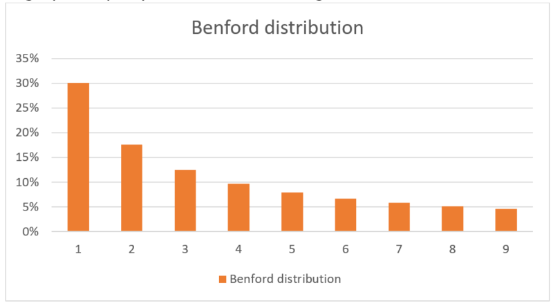
Shown to be applicable to a wide array of data, from population numbers and electricity bills to surface areas of all rivers in the world, it has been successfully applied as an aid in accounting fraud detection. People who make up figures tend to distribute their digits fairly uniformly. This means that all else equal, accounting statements that have been tampered with will deviate from Benford’s Law more than those that have not.
Here are two illustrative examples of Benford’s distribution at work. I decided to compare two companies’ financial statements against Benford’s Law. One company is the American IT giant Microsoft, a company scrutinized by the public and dozens of analysts and sure to be relatively straightforward in its accounting practices. Here is Microsoft’s first-digit distribution plotted against Benford’s:
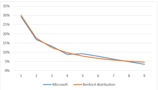
Notice that although the fit is imperfect, it is a very close one and enforces our initial hypothesis about MSFT being a decent company in terms of the absence of accounting malpractice.
As a second example, I decided to take a certain Russian private company that I knew prepared fraudulent accounting statements, showing rubbish, next-to-zero profits on its books while the owner siphoned off all the cash into rogue firms controlled by persons close to him. This was done because the Russian Ministry of Defense, who was the main customer of this company, had very strict regulations about the profit margins not exceeding certain levels. So instead of lowering his appetite, the owner overstated expenses, undoubtedly not without the help of his patrons within the Ministry itself. Here is the distribution for this company:
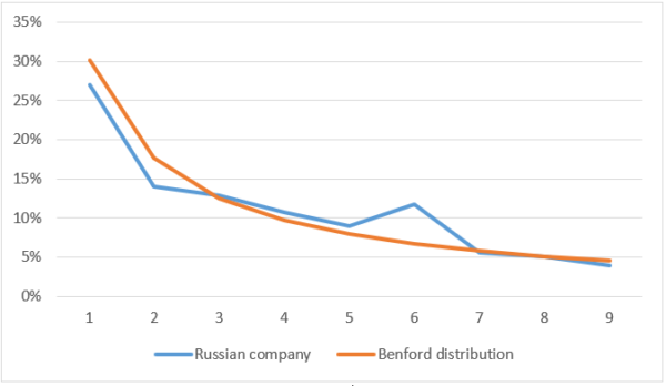
The visuals speak for themselves.
For all the financial data for each company and year, I calculate the mean absolute deviations of the frequency of the first digits from Benford’s distribution. I then divide the dataset into quartiles and take as a positive signal if the firm’s score is equal to or below the second quartile.
While the Benford score is applied as an unconditional shift, the other seven variables are binary and are added up. A company scores high if it passes the Benford test and fulfills the conditions of 6 or 7 other variables.
Global Results
The table below summarizes the results of the backtested strategy on the global universe of stocks (equal-weighted):
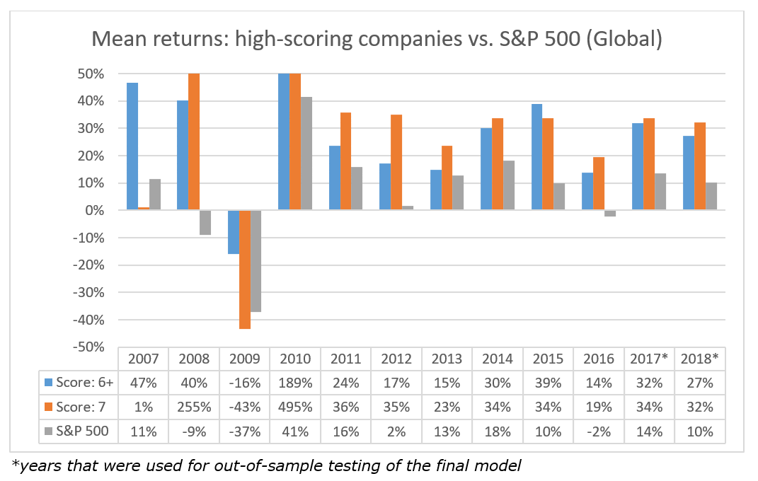
Scores 6+ and 7 can be thought as analogous to scoring an 8+ or 9 in Piotroski’s system. The number of stocks that were picked by the respective strategies:

The list of actual stocks that made it into the portfolios, along with their country and industry, will be presented in the Appendix.
European Union Results(20)
Here are the results for European countries:
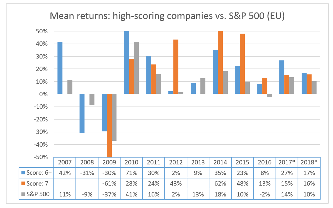
Empty cells mean that no companies among European ones were chosen for the portfolio since scoring a “seven” presumes passing a very strict set of criteria, just like scoring a “nine” on Piotroski(21).

Industry-wise and Country-wise Composition
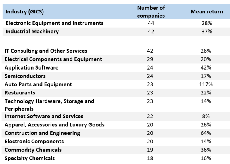
To give a sense of what industries and countries the model picks up, I compiled two lists, based on the global model with criteria set to 6+.
Top 15 industries that were chosen over 2006-2017 (score 6+), number of companies, and average 1-year forward return:
Top 15 countries that were chosen over 2006-2017 (score 6+), number of companies and average 1-year forward return:
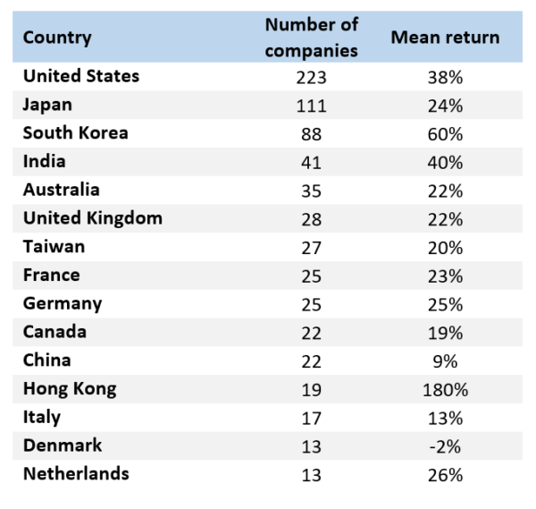
For all industries and for all countries except one, the returns are strongly positive. This further serves as proof that the strategy is balanced and statistically significant, retaining its significance across industries and most countries. A promising thing to test in the future could be whether certain countries or industries should be left out while others have given more weight, however, that presupposes taking a macro-view, a trait this particular strategy tried to explicitly avoid when adjusting BVIC/MVIC, so caution should be taken.
If you would like to receive a list of companies that made it into the portfolios, please contact the author at [email protected].
References[+]
| ↑1 | Showing that EMH proponents are forced to add on more factors to their models to prove that the market is efficient and sustainable alpha is impossible. |
|---|---|
| ↑2 | Upon addition of each new factor to the model, misclassified data is given more weight than that which has been classified correctly, thus forcing the procedure to look for a next factor that will address the instances of misclassified data. For example, I gave more weight to years that underperformed the market. |
| ↑3 | Data includes 198 variables relating to the Income Statement (IS), Balance Sheet (BS), and Statement of Cash Flows (CF) of each company as well as additional variables such as volatility data, EBITDA, EV, Market cap and several others. |
| ↑4 | This proves that the results are not driven by emerging or developing markets premia. |
| ↑5 | Like “brute force generators”, to borrow an analogy from the sphere of IT. |
| ↑6 | Its simplicity has been questioned by Piotroski himself, who rightly notes that the success of a simple strategy of buying high B/M stocks relies heavily on the outperformance of a few “star” stocks. Statistically speaking, the high B/M universe is skewed to the right in terms of returns distribution. |
| ↑7 | This metric was proposed by Shannon Pratt, author of some of the best guides for valuation practitioners, “Valuing a Business” and “Cost of Capital” to name a couple. |
| ↑8 | A tercile is formed when all data are sorted from largest to smallest and then separated into three segments of equal size. This procedure has to be done manually in MS Excel for lack of a =TERCILE() function. |
| ↑9 | Here, the median is used instead of the mean because it is a more stable metric, less dependent on outliers and the irregularities in the shape of the distribution |
| ↑10 | Mohanram, P. S. Separating Winners from Losers among Low Book-to-Market Stocks using Financial Statement Analysis (2005) |
| ↑11 | Penman, Stephen H. and Zhang, Xiao-Jun, Accounting Conservatism, the Quality of Earnings, and Stock Returns (December 1999) |
| ↑12 | Four segments of equal size, i.e. with the same number of stocks in each. |
| ↑13 | One might ask why this variable was calculated as “decrease in CA” instead of “decrease in non-cash CA”. This is because some firms are “sitting on their cash”. For these firms, growth in cash is not necessarily a good thing. Moreover, while their cash may be increasing and their non-cash CA may be decreasing, they will not show up as positive on the “decrease in CA” variable since cash usually represents the bulk of their CA – this can be thought of as penalization for such firms. |
| ↑14 | Here we assume, together with Prof. Piotroski, that most value firms, either measured as high B/M, or as high BVIC/MVIC, are prone to be financially distressed. |
| ↑15 | To be fair, a company may be incentivized to understate its profits for tax management purposes. Such a company’s asset base will quickly become inadequately small on the books and the adequacy of the company’s level of fixed assets is addressed by one of the variables, FA/Sales Q-score. In addition, such a situation will result in a large tax outflow when the asset is disposed of at a price much higher than its residual value. |
| ↑16 | This is a bit oversimplified since we are not accounting for inflation, which would mean that the actual average CAPEX/D&A ratio across the market should be slightly higher than one. |
| ↑17 | Defined as the industry median, see description of Q-score (type three variables). |
| ↑18 | The period for RSI calculation is usually 14 days. |
| ↑19 | https://en.wikipedia.org/wiki/Benford’s_law |
| ↑20 |
I consulted with this list to define European countries: https://en.wikipedia.org/wiki/List_of_European_countries_by_population with two notable exclusions being Russia and Ukraine (high probability of creative accounting) |
| ↑21 | It is notable that if one goes to the site of American Association of Individual Investors, which ranks the most popular stock-picking systems (here: https://www.aaii.com/stockideas/performance) and downloads monthly data, for the past five or so years there will be mostly “0.0%” returns for “Piotroski 9” strategy. I contacted AAII and they confirmed that it means no stocks pass all the nine criteria. |
About the Author: Mikhail Subbotin
—
Important Disclosures
For informational and educational purposes only and should not be construed as specific investment, accounting, legal, or tax advice. Certain information is deemed to be reliable, but its accuracy and completeness cannot be guaranteed. Third party information may become outdated or otherwise superseded without notice. Neither the Securities and Exchange Commission (SEC) nor any other federal or state agency has approved, determined the accuracy, or confirmed the adequacy of this article.
The views and opinions expressed herein are those of the author and do not necessarily reflect the views of Alpha Architect, its affiliates or its employees. Our full disclosures are available here. Definitions of common statistics used in our analysis are available here (towards the bottom).
Join thousands of other readers and subscribe to our blog.

