1. Introduction
Part 1 of this analysis, which is available here, examines filters modeled on second-order processes from a digital signal processing (DSP) perspective to illustrate their properties and limitations. To briefly recap, a time series based on a second-order process consists of a mean a and a linear trend b which is contaminated with random normally distributed noise ε(t) where ε(t) ~ N(0, σε2):
- second-order process – mean a and linear trend b: x(t) = a + b*t + ε(t)
The filters analyzed in Part 1 include double moving average, double linear weighted moving average, double exponential smoothing, and alpha-beta tracking filters. Part 2 extends the analysis to filters modeled on third-order processes. A third-order process consists of a mean a, a linear trend b, and a quadratic trend c which is contaminated with random normally distributed noise ε(t):
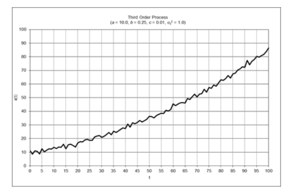
- third-order process – mean a, linear trend b, and quadratic trend c: x(t) = a + b*t + ½*c*t2 + ε(t)
The filters analyzed are triple moving average, triple linear weighted moving average, triple exponential smoothing, and alpha-beta-gamma tracking filters. Note: This article assumes familiarity with Part 1 and also with the characteristics of financial time series and the digital signal processing concepts discussed in “An Introduction to Digital Signal Processing for Trend Following”, which is available here.
2. Triple Moving Average (TMA)
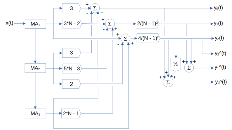
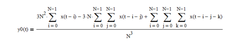
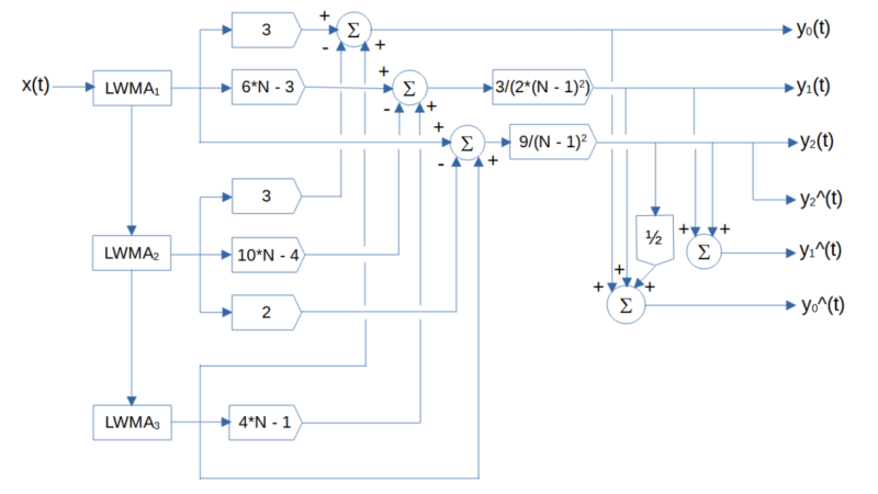
Triple moving average (TMA) is a time series forecasting and process control method that uses three single moving averages to estimate time series that contain linear and quadratic trends(1). The triple moving average set of equations is:

where N is the number of input data points, i.e., the moving average length N (N > 1), included in the three single moving averages used to calculate the triple moving average, and x(t) represents the price at integer time t.
The triple moving average generates five main outputs: an estimate of the mean y0(t) at time step t, an estimate of the linear trend y1(t) at time step t, an estimate of the quadratic trend y2(t) at time step t, a mean prediction y0^(t) made at time step t for the next time step t+1, and a linear trend prediction y1^(t) made at time step t for the next time step t+1. The quadratic trend prediction y2^(t) for the next time step t+1 is the same as the quadratic trend estimate y2(t) since a triple moving average does not model cubic and higher-order trends.
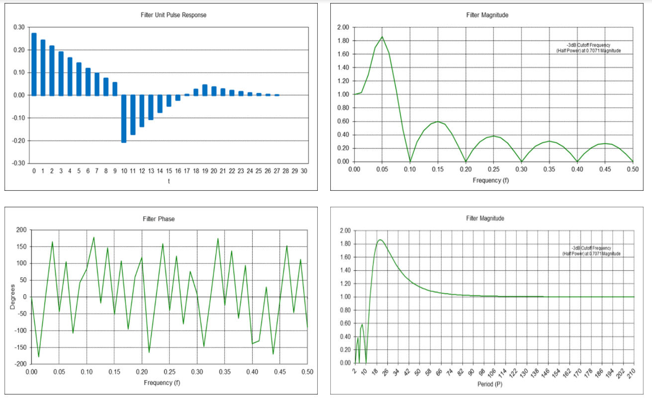
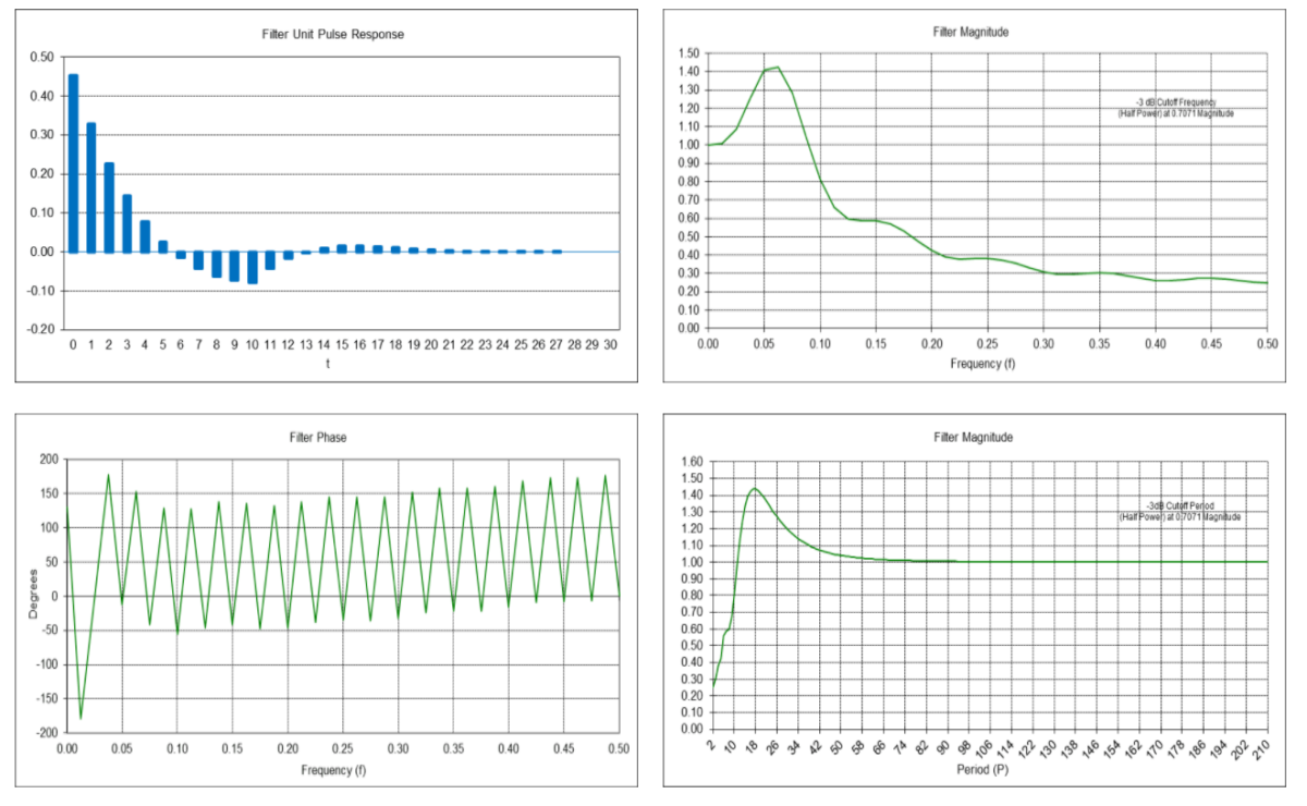
Triple Moving Average Mean Filter Frequency Response (N = 10)
The triple moving average mean filter y0(t) is a type of FIR low pass filter, i.e., it passes frequencies below the cutoff frequency fc and attenuates frequencies above the cutoff frequency. The value N determines the cutoff frequency, which is inversely proportional to N (the cutoff period Pc is proportional to N). The filter coefficients sum to 1.0.
FIR mean filter difference equation:
Example: Triple moving average mean filter with length N = 10
Passes frequencies below the -3 dB (half power) cutoff frequency fc of approximately 0.0824, which corresponds to a cutoff period Pc of approximately 12 time samples. Completely suppresses frequencies of 0.1, 0.2, 0.3, 0.4, and 0.5, which correspond to periods of 10, 5, 3.3333, 2.5, and 2 time samples, respectively. (Suppression occurs because, for example, the average value of a 10 time-sample period sine wave over 10 time samples is zero, the average value of two 5 time-sample period sine waves over 10 time samples is zero, etc.) There is a magnitude peak above 1.0 (i.e., 0 dB) at a period of approximately 21 time samples.
Triple Moving Average Linear Trend Filter Frequency Response (N = 10)
The triple moving average linear trend filter y1(t) is a type of FIR bandpass filter. The filter has a center (also called “resonant”) frequency f0, corresponding to a center period P0, which passes at maximum power. The value N determines the center frequency f0, which is inversely proportional to N (the center period P0 is proportional to N). The filter coefficients sum to 0.0.
FIR linear trend filter difference equation:
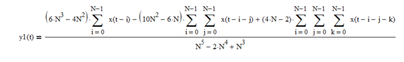
Example: Triple moving average linear trend filter with length N = 10
The center frequency f0 is approximately 0.05, which corresponds to a center period P0 of approximately 20 time samples. The filter completely suppresses frequencies of 0.1, 0.2, 0.3, 0.4, and 0.5, which correspond to periods of 10, 5, 3.333, 2.5, and 2 time samples, respectively.
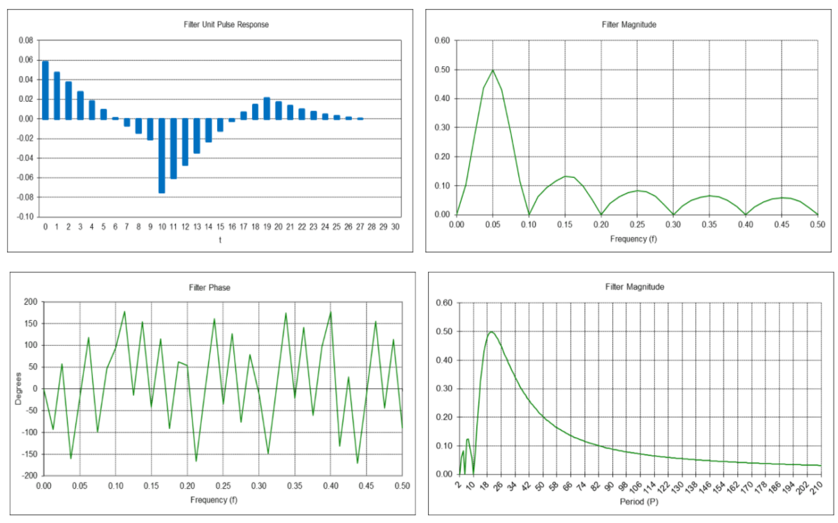
Triple Moving Average Quadratic Trend Filter Frequency Response (N = 10)
The triple moving average quadratic trend filter y2(t) is a type of FIR bandpass filter. The filter has a center (also called “resonant”) frequency f0, corresponding to a center period P0, which passes at maximum power. The value N determines the center frequency f0, which is inversely proportional to N (the center period P0 is proportional to N). The filter coefficients sum to 0.0.
FIR quadratic trend filter difference equation:
Example: Triple moving average quadratic trend filter with length N = 10
The center frequency f0 is approximately 0.5, which corresponds to a center period P0 of approximately 20 time samples. The filter completely suppresses frequencies of 0.1, 0.2, 0.3, 0.4, and 0.5, which correspond to periods of 10, 5, 3.333, 2.5, and 2 time samples, respectively.
Triple Moving Average Mean, Linear Trend, and Quadratic Trend Filter Example
The following price chart of the daily S&P 500 stock index closing values for 2018 and 2019, which includes 503 trading days, shows the triple moving average mean (dashed blue line), linear trend (solid blue line), and quadratic trend (solid green line) for filter length N = 10. The single moving average mean (dashed red line) for filter length N = 10 is shown for comparison.
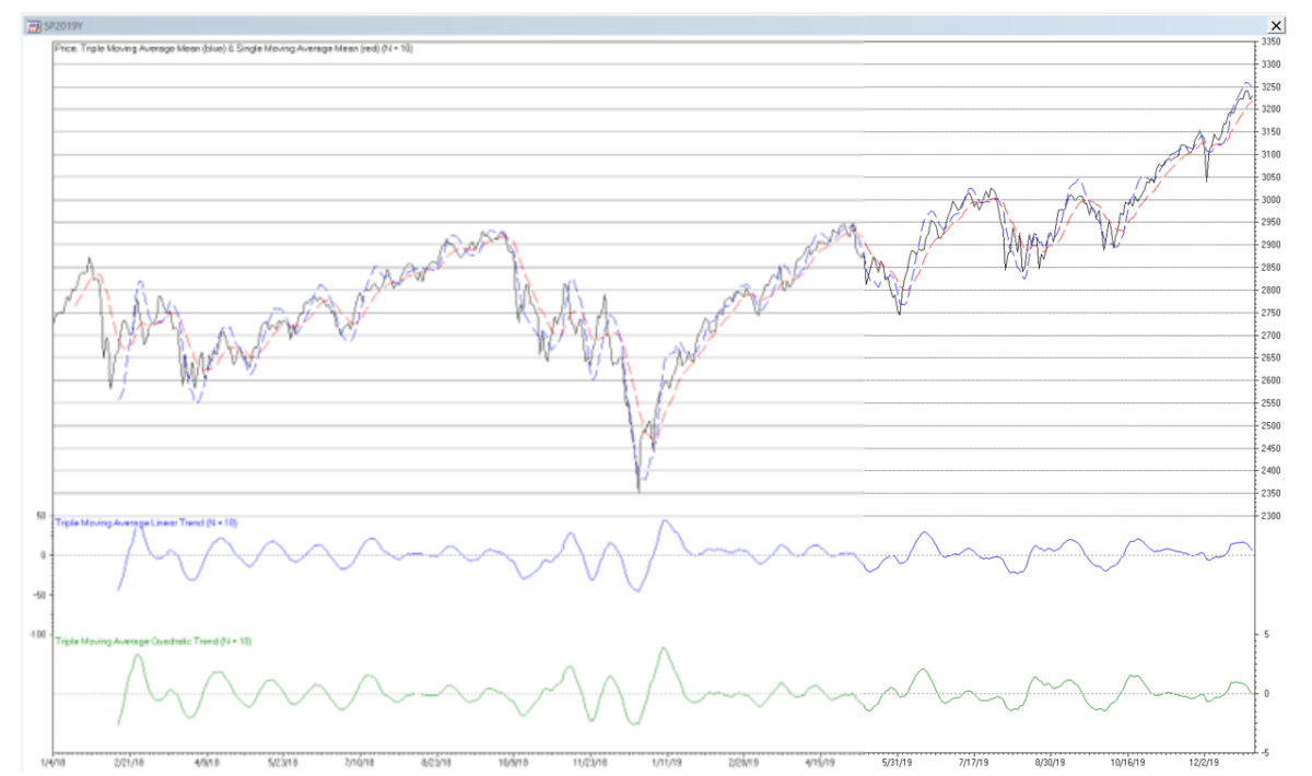
The results are hypothetical results and are NOT an indicator of future results and do NOT represent returns that any investor actually attained. Indexes are unmanaged, do not reflect management or trading fees, and one cannot invest directly in an index.
The amplitude of the linear trend filter output is proportional to the local slope of the price, i.e., the greater the amplitude, the steeper the slope. Similarly, the amplitude of the quadratic trend filter output is proportional to the local slope of the linear trend. However, the output of both filters can be affected by the presence of cycles and higher order trends.
Trading Signal Generation
Trading signals using triple moving average mean, linear trend, and quadratic trend filters can potentially be generated, for example, when:
- the price crosses above (buy) or below (sell) the mean line
- the mean line reaches a local crest (sell) or trough (buy)
- the linear trend line crosses above (buy) or below (sell) the zero line
- the linear trend line reaches a local crest (sell) or trough (buy)
- the quadratic trend line crosses above (buy) or below (sell) the zero line
- the quadratic trend line reaches a local crest (sell) or trough (buy)
or by a combination of these conditions.
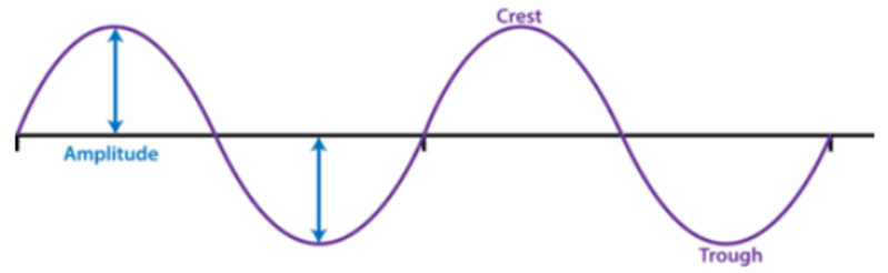
The graph below illustrates the concepts of amplitude, crest, and trough:
3. Triple Linear Weighted Moving Average (TLWMA)
Triple linear weighted moving average (TLWMA) is a modified form of the triple moving average that uses linear weighted moving averages instead of moving averages to estimate the mean, linear trend, and quadratic trend. The triple linear weighted moving average set of equations is:

where N is the number of input data points, i.e., the linear weighted moving average length N (N > 1), included in the three single linear weighted moving averages used to calculate the triple linear weighted moving average, and x(t) represents the price at integer time t.
The triple linear weighted moving average generates five main outputs: an estimate of the mean y0(t) at time step t, an estimate of the linear trend y1(t) at time step t, an estimate of the quadratic trend y2(t) at time step t, a mean prediction y0^(t) made at time step t for the next time step t+1, and a linear trend prediction y1^(t) made at time step t for the next time step t+1. The quadratic trend prediction y2^(t) for the next time step t+1 is the same as the quadratic trend estimate y2(t), since a triple linear weighted moving average does not model cubic and higher-order trends.
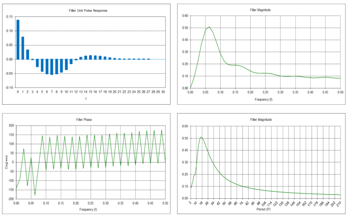
Triple Linear Weighted Moving Average Mean Filter Frequency Response (N = 10)
The triple linear weighted moving average mean filter y0(t) is a type of FIR low pass filter. The value N determines the cutoff frequency, which is inversely proportional to N (the cutoff period Pc is proportional to N). The filter coefficients sum to 1.0.
FIR mean filter difference equation:

Example: Triple linear weighted moving average mean filter with length N = 10
Passes frequencies below the -3 dB (half power) cutoff frequency fc of approximately 0.1075, which corresponds to a cutoff period Pc of approximately 9.3 time samples. There is a magnitude peak above 1.0 (i.e., 0 dB) at a period of approximately 17 time samples.
Triple Linear Weighted Moving Average Linear Trend Filter Frequency Response (N = 10)
The triple linear weighted moving average linear trend filter y1(t) is a type of FIR bandpass filter. The value N determines the center frequency f0, which is inversely proportional to N (the center period P0 is proportional to N). The filter coefficients sum to 0.0.
FIR linear trend filter difference equation:

Example: Triple linear weighted moving average linear trend filter with length N = 10
The center frequency f0 is approximately 0.0588, which corresponds to a center period P0 of approximately 17 time samples.
Triple Linear Weighted Moving Average Quadratic Trend Filter Frequency Response (N = 10)
The triple linear weighted moving average quadratic trend filter y2(t) is a type of FIR bandpass filter. The value N determines the center frequency f0, which is inversely proportional to N (the center period P0 is proportional to N). The filter coefficients sum to 0.0.
FIR quadratic trend filter difference equation:
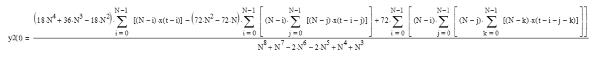
Example: Triple linear weighted moving average quadratic trend filter with length N = 10
The center frequency f0 is approximately 0.0625, which corresponds to a center period P0 of approximately 16 time samples.
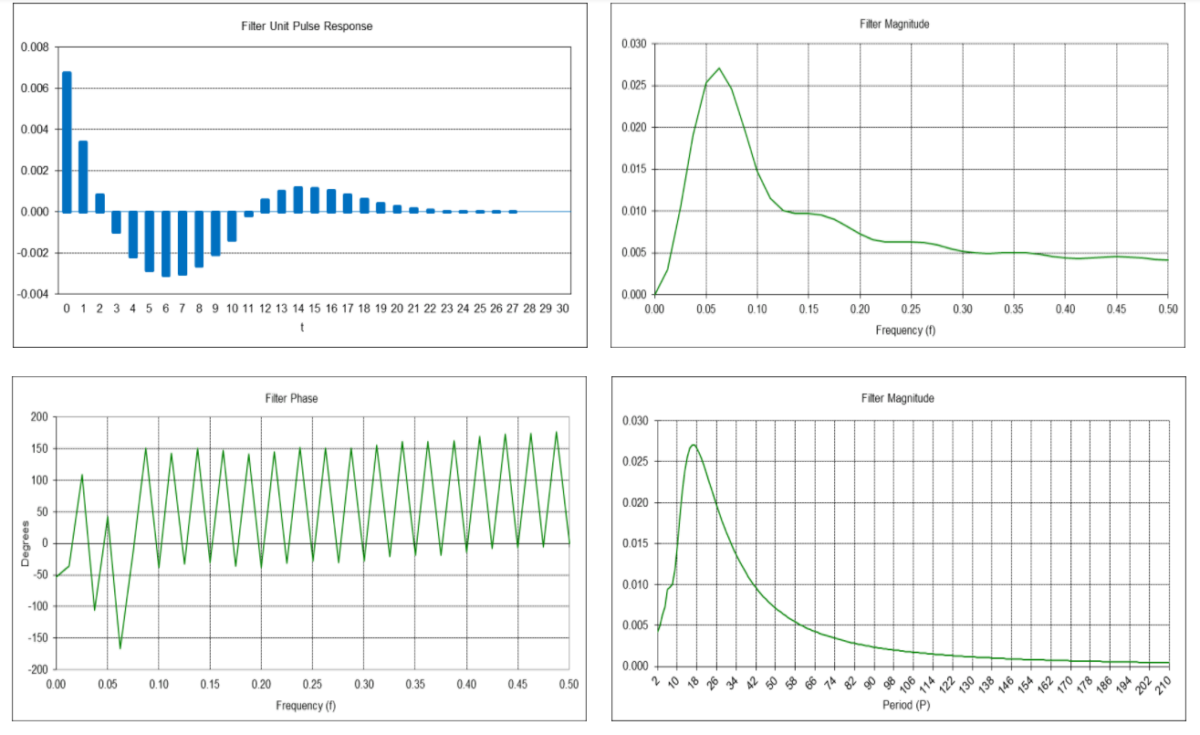
Triple Linear Weighted Moving Average Mean, Linear, and Quadratic Trend Filter Example
The following S&P 500 daily price chart shows the triple linear weighted moving average mean (dashed blue line), linear trend (solid blue line), and quadratic trend (solid green line) for filter length N = 10. The single linear weighted moving average mean (dashed red line) for filter length N = 10 is shown for comparison.
Trading signals using triple linear weighted moving average mean, linear trend, and quadratic trend filters can potentially be generated in a similar manner to those described for triple moving average mean, linear trend, and quadratic trend filters.
4. Triple Exponential Smoothing (TES)
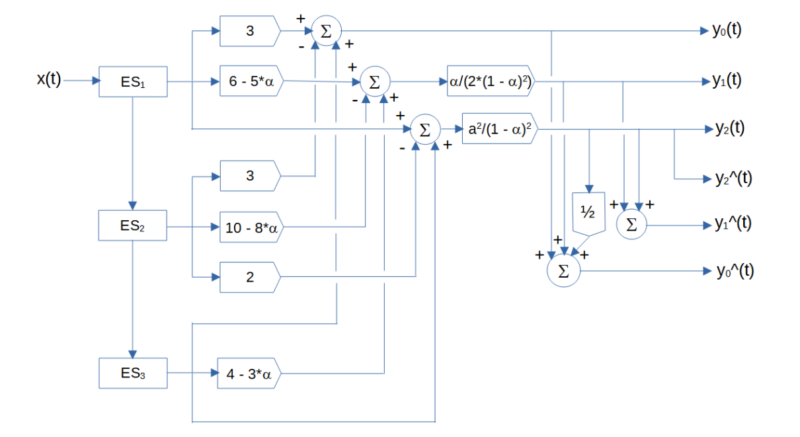
Triple exponential smoothing (TES) is similar to the triple moving average, except that it uses exponential smoothing instead of moving averages to estimate the mean, linear trend, and quadratic trend(2). The triple exponential smoothing set of equations is:

where α is the exponential smoothing constant (0 <= α <= 1) used in the three single exponential smoothings used to calculate the triple exponential smoothing and x(t) represents the price at integer time t.
Triple exponential smoothing generates five main outputs: an estimate of the mean y0(t) at time step t, an estimate of the linear trend y1(t) at time step t, an estimate of the quadratic trend y2(t) at time step t, a mean prediction y0^(t) made at time step t for the next time step t+1, and a linear trend prediction y1^(t) made at time step t for the next time step t+1. The quadratic trend prediction y2^(t) for the next time step t+1 is the same as the quadratic trend estimate y2(t), since triple exponential smoothing does not model cubic and higher order trends.
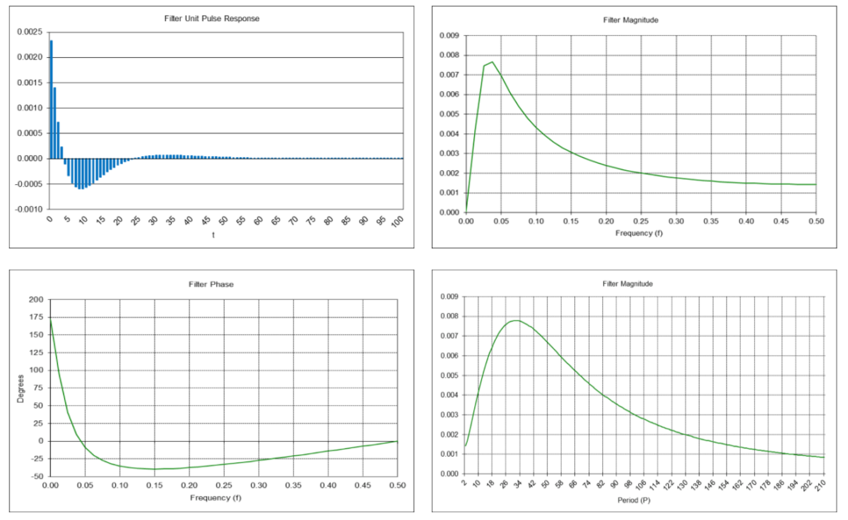
Triple Exponential Smoothing Mean Filter Frequency Response (α = 0.1325)
The triple exponential smoothing mean filter y0(t) is a type of IIR low pass filter. The value of the exponential smoothing constant α determines the cutoff frequency, which is proportional to α (the cutoff period Pc is inversely proportional to α).
IIR mean filter difference equation (requires proper initialization):
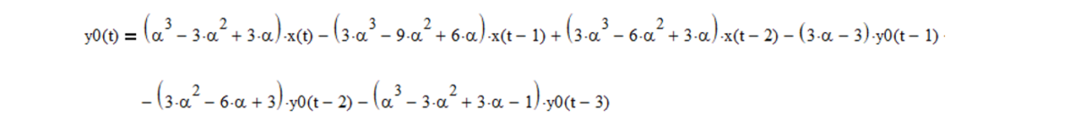
Example: Triple exponential smoothing mean filter with exponential smoothing constant α = 0.1325
The filter has about the same -3 dB (half power) cutoff frequency fc of approximately 0.0824 (cutoff period Pc of approximately 12 time samples) as a triple moving average filter with length N = 10. There is a magnitude peak above 1.0 (i.e., 0 dB) at a period of approximately 40 time samples.
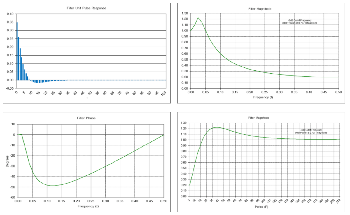
Triple Exponential Smoothing Linear Trend Filter Frequency Response (α = 0.1325)
The triple exponential smoothing linear trend filter y1(t) is a type of IIR bandpass filter. The value of the exponential smoothing constant α determines the center frequency f0, which is proportional to α (the center period P0 is inversely proportional to α).
IIR linear trend filter difference equation (requires proper initialization):

Example: Triple exponential smoothing linear trend filter with exponential smoothing constant α = 0.1325
The center frequency f0 is approximately 0.0303, which corresponds to a center period P0 of approximately 33 time samples.
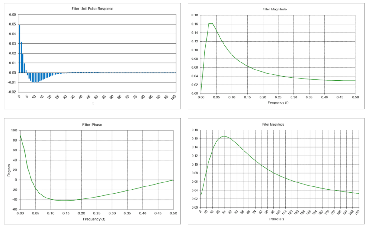
Triple Exponential Smoothing Quadratic Trend Filter Frequency Response (α = 0.1325)
The triple exponential smoothing quadratic trend filter y2(t) is a type of IIR bandpass filter. The value of the exponential smoothing constant α determines the center frequency f0, which is proportional to α (the center period P0 is inversely proportional to α).
IIR quadratic trend filter difference equation:

Example: Triple exponential smoothing quadratic trend filter with exponential smoothing constant α = 0.1325
The center frequency f0 is approximately 0.0323, which corresponds to a center period P0 of approximately 31 time samples.
Triple Exponential Smoothing Mean, Linear Trend, and Quadratic Trend Filter Example
The following S&P 500 daily price chart shows the triple exponential smoothing mean (dashed blue line), linear trend (solid blue line), and quadratic trend (solid green line) with smoothing constant α = 0.1325. The single exponential smoothing mean (dashed red line) with smoothing constant α = 0.1325 is shown for comparison.
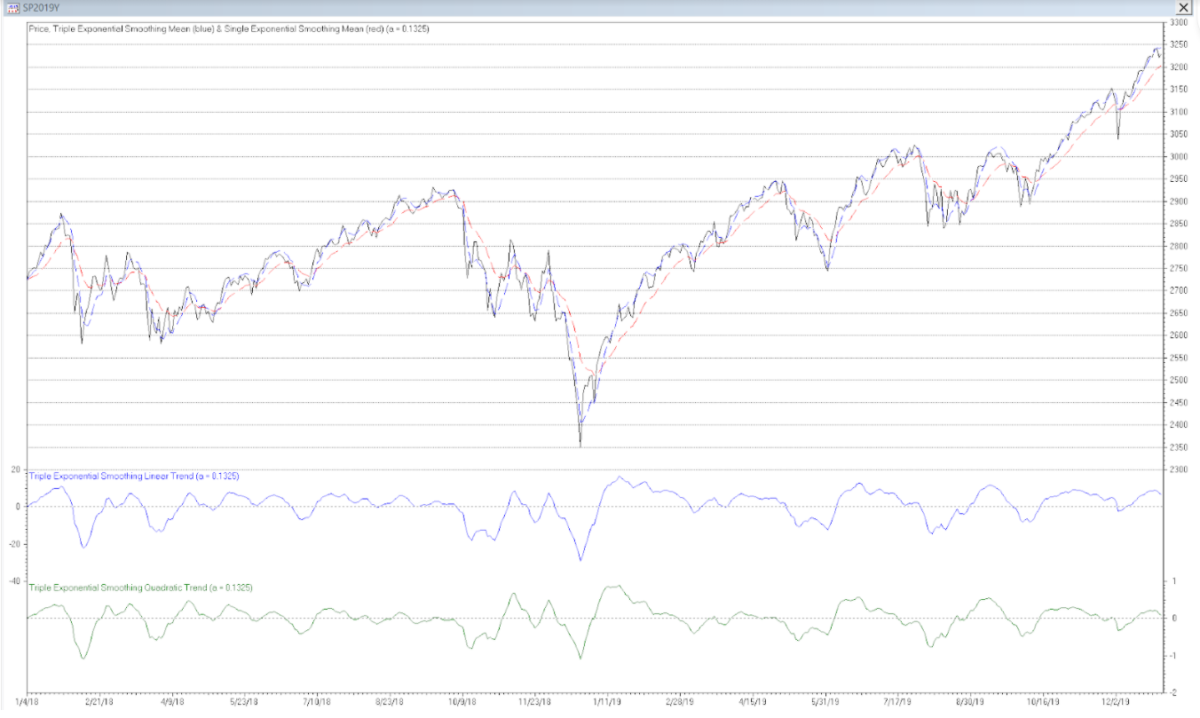
Trading signals using triple exponential smoothing mean, linear trend, and quadratic trend filters can potentially be generated in a similar manner to those described for triple moving average mean, linear trend, and quadratic trend filters.
5. Alpha-Beta-Gamma (α−β−γ) Tracking Filter
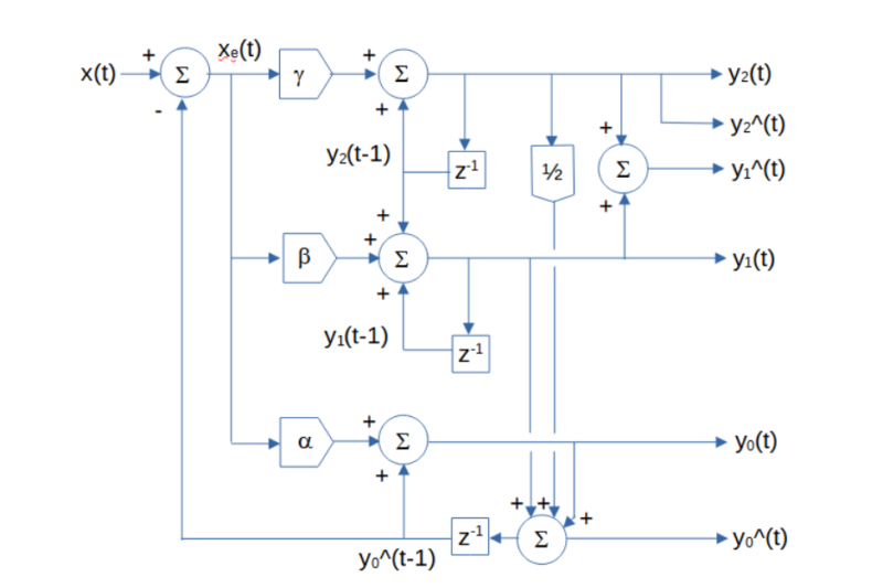
The alpha-beta-gamma (α−β−γ) filter is used for object tracking in track-while-scan radar systems, based on an acceleration motion model(3)(4). The function of the tracking filter is to process noisy position measurement inputs into “smoothed” position, velocity, and acceleration estimate outputs. The alpha-beta-gamma tracking filter set of equations is:

where α is the position smoothing constant, β is the velocity smoothing constant, γ is the acceleration smoothing constant, and x(t) is the observed position of the object (or price in this case) at integer time t. Note that the alpha-beta-gamma filter position estimate is analogous to the mean estimate, the velocity estimate is analogous to the linear trend estimate, and the acceleration estimate is analogous to the quadratic trend estimate of the other filters described above. The α, β, and γ smoothing constants are subject to the following stability constraints:
![]()
The alpha-beta-gamma tracking filter generates five main outputs: an estimate of the position y0(t) at time step t, an estimate of the velocity y1(t) at time step t, an estimate of the acceleration y2(t) at time step t, a position prediction y0^(t) made at time step t for the next time step t+1, and a velocity prediction y1^(t) made at time step t for the next time step t+1. The acceleration prediction y2^(t) for the next time step t+1 is the same as the acceleration estimate y2(t), since the alpha-beta-gamma tracking filter does not model jerk and higher order maneuvers.
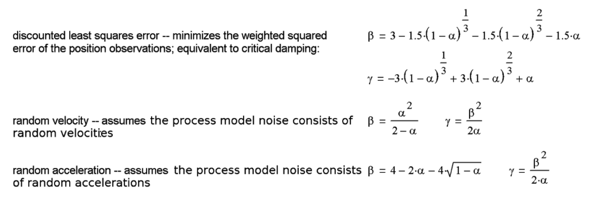
Various alpha-beta-gamma filter smoothing constant relationship equations have been developed to calculate optimal values, based on an assumed underlying process model that approximates the dynamic behavior of the target or on a set of filter design objectives, such as providing good transient response and small noise and prediction error(5)(6). They include:
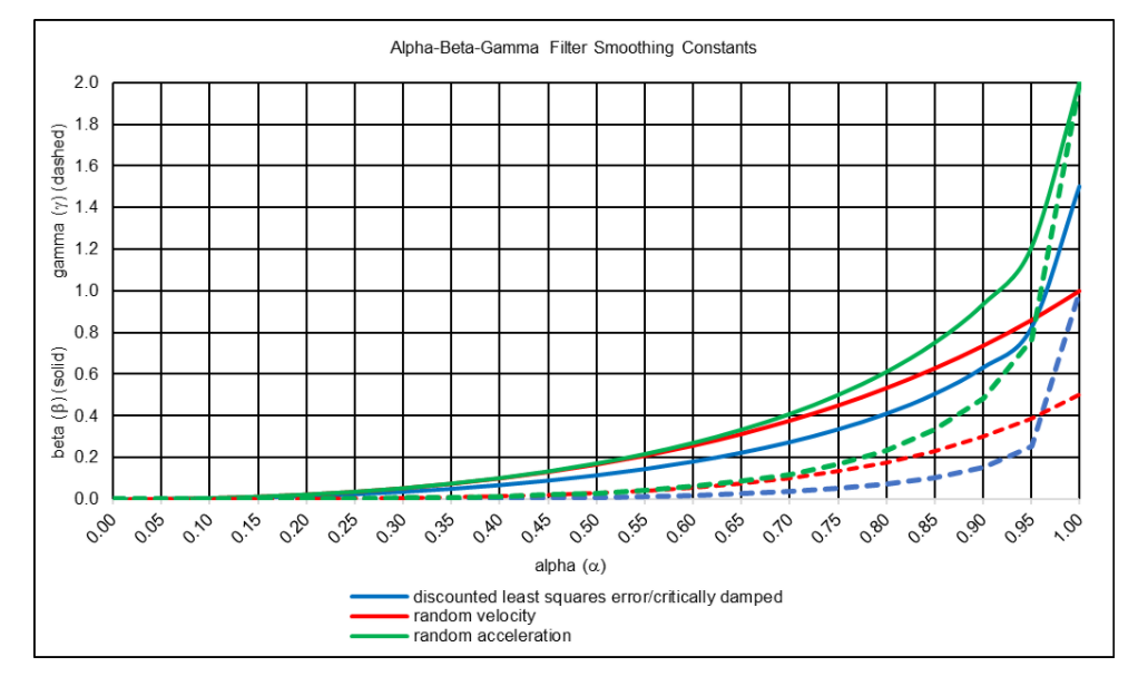
Notes:
- Discounted least squares error (critically damped) smoothing constants α, β, and γ produce results equivalent to triple exponential smoothing if

where α3 is the triple exponential smoothing constant.
- The alpha-beta-gamma tracking filter is closely related to the three-state steady-state Kalman filter, where the three states are position, velocity, and acceleration(7).
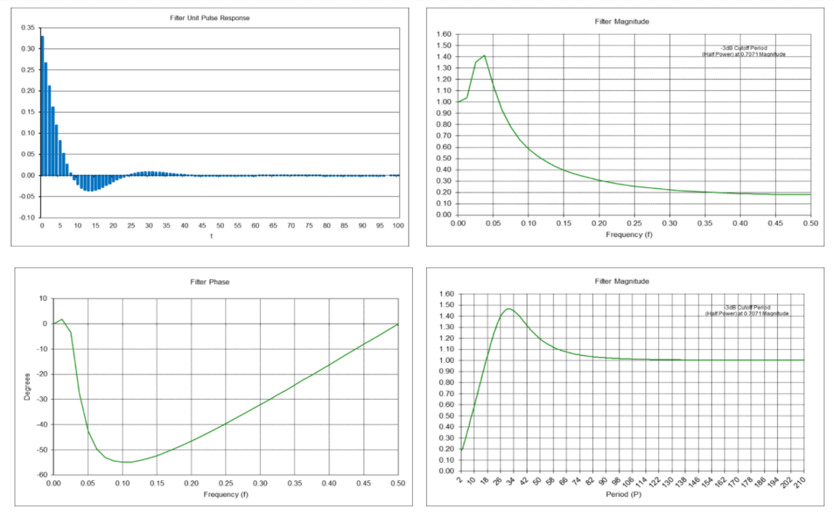
Alpha-Beta-Gamma Position Tracking Filter Frequency Response (α = 0.3289, β = 0.0654, γ = 0.0065)
The alpha-beta-gamma position tracking filter y0(t) is a type of IIR low pass filter. The α, β, and γ smoothing constant values determine the cutoff frequency of the filter.
IIR position tracking filter difference equation (requires proper initialization):

Example: Alpha-beta-gamma position tracking filter using random acceleration-based smoothing constants α = 0.3289, β = 0.0654, and γ = 0.0065
The filter has a -3 dB (half power) cutoff frequency fc of approximately 0.0824 (cutoff period Pc of approximately 12 time samples), similar to that of a triple moving average mean filter with length N = 10. There is a magnitude peak above 1.0 (i.e., 0 dB) at a period of approximately 31 time samples.
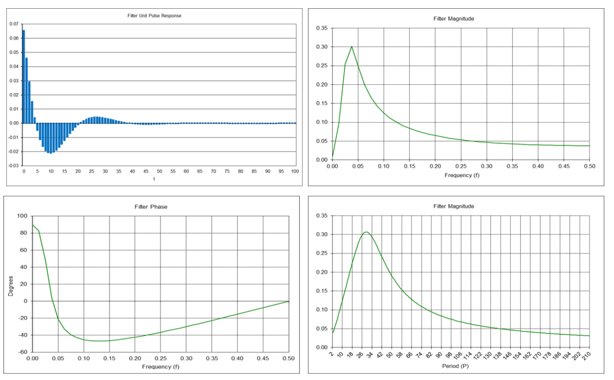
Alpha-Beta-Gamma Velocity Tracking Filter Frequency Response (α = 0.3289, β = 0.0654, γ = 0.0065)
The alpha-beta-gamma velocity tracking filter y1(t) is a type of IIR bandpass filter. The α, β, and γ smoothing constant values determine the center frequency f0 of the filter.
IIR velocity tracking filter difference equation (requires proper initialization):

Example: Alpha-beta-gamma velocity tracking filter using random acceleration-based smoothing constants α = 0.3289, β = 0.0654, and γ = 0.0065
The center frequency f0 is approximately 0.0345, which corresponds to a center period P0 of approximately 29 time samples.
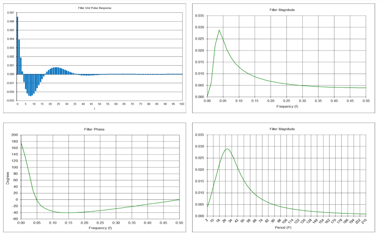
Alpha-Beta-Gamma Acceleration Tracking Filter Frequency Response (α = 0.3289, β = 0.0654, γ = 0.0065)
The alpha-beta-gamma acceleration tracking filter y2(t) is a type of IIR bandpass filter. The α, β, and γ smoothing constant values determine the center frequency f0 of the filter.
IIR acceleration tracking filter difference equation (requires proper initialization):

Example: Alpha-beta-gamma acceleration tracking filter using random acceleration-based smoothing constants α = 0.3289, β = 0.0654, and γ = 0.0065
The center frequency f0 is approximately 0.0357, which corresponds to a center period P0 of approximately 28 time samples.
Random Acceleration-Based Alpha-Beta-Gamma Position, Velocity, and Acceleration Tracking Filter Example
The following S&P 500 daily price chart shows the alpha-beta-gamma position (dashed blue line), velocity (solid blue line), and acceleration (solid green line) tracking filters using random acceleration-based smoothing constants α = 0.3289, β = 0.0654, and γ = 0.0065.
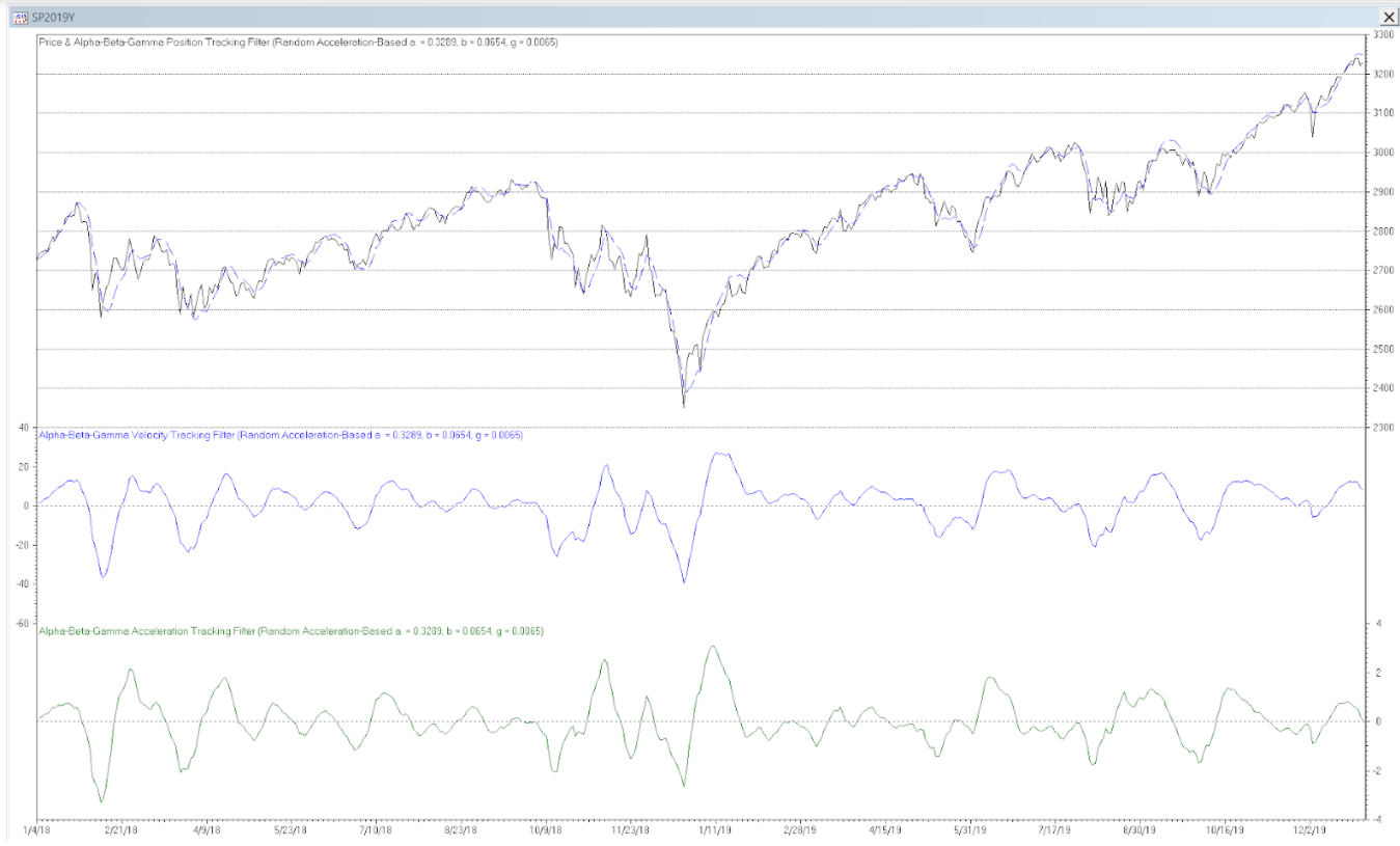
Trading signals using alpha-beta-gamma position, velocity, and acceleration tracking filters can potentially be generated in a similar manner to those described for triple moving average mean, linear trend, and quadratic trend filters.
6. Prediction and Prediction Accuracy
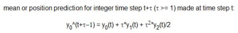
For a time series with an underlying third-order process, assuming that the current quadratic trend (acceleration) y2(t) is locally constant and using the same time step convention as is used for the one time-step predictions above, mean (position) predictions y0^ at future integer time steps can be made at time step t, using the following equation:
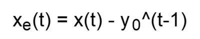
One measure that can be used to evaluate the appropriate filter length or smoothing constant values to use with a particular time series is to calculate the root mean square error (RMSE) of the one time-step predictions of the filter over a sample of observations. The one time-step prediction error xe(t) at each time step t is the difference between the input value x(t) at time step t and the prediction y0^(t-1) made for time step t at the previous time step t-1:
The root mean square error over a sample of N observations is:

In general, the filter length or smoothing constant values that produce the minimum RMSE can be helpful in determining a useful setting. Unlike filters that are modeled on first order processes, filters modeled on third order processes will usually have a non-trivial minimum RMSE value when applied to financial time series. However, values that minimize RMSE may not necessarily correspond to maximum trading profitability. In addition, the value that minimizes RMSE in one sample of observations will not necessarily be the same in a different sample, due to the volatility, non-normality, and non-stationarity usually observed in financial time series.
7. General Comments on Third Order Process Filters
While mean (position) filters modeled on third order processes are able to follow input time series that contain a locally constant quadratic trend (acceleration) with less lag compared to filters modeled on first or second order processes, if the input time series contains cubic or higher order trends (jerk or higher order target maneuvers), for example, third order mean (position) filter estimates will lag the input.
Filters modeled on fourth or higher order underlying processes can also be used, but filters modeled on second or third order processes are usually sufficient to capture the significant trends in most financial time series.
Third order process linear trend (velocity) and quadratic trend (acceleration) filters are bandpass filters which are “tuned” to a specific center frequency or period, based on the filter coefficients, with an associated phase response. As a result, if the input time series contains a cycle with a period that is less than the center period of the filter, the filter output will crest (trough) after the input time series cycle crest (trough). Conversely, if the input time series cycle period is greater than the center period, the filter output will crest (trough) before the input time series crest (trough). This behavior can be observed in the linear and quadratic trend and in the velocity and acceleration filter outputs in the S&P 500 daily price charts.
Since financial time series are non-stationary with means and variances that change over time, the use of filters with fixed parameters will not perform well at all times for trading purposes. As a result, filter coefficients that are “fitted” to a particular portion of a time series history will not necessarily produce good results in the future.
Acknowledgements
I would like to thank Larry Stabile for reviewing this article and providing many helpful comments and suggestions.
Appendix – Equation Set Derivations
The derivation of the triple moving average, triple linear weighted moving average, and triple exponential smoothing sets of equations is mathematically complex and beyond the scope of this article.
For reference, the proof of the “fundamental theorem of exponential smoothing”, which includes that for double, triple, and higher-order exponential smoothing, can be found in(8). The proof can be extended to double, triple, and higher-order moving averages by substituting the following for α in the equations, where N is the single moving average length:
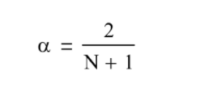
Similarly, the proof can be extended to double, triple, and higher order linear weighted moving averages by substituting the following for α in the equations, where N is the single linear weighted moving average length:
These substitutions equate the average age of the data included in exponential smoothing to the average age of the data included in the corresponding moving average and linear weighted moving average.

References[+]
| ↑1 | Brown, R. G., Smoothing, Forecasting, and Prediction of Discrete Time Series, Prentice Hall, 1962. |
|---|---|
| ↑2 | Brown, R. G., Smoothing, Forecasting, and Prediction of Discrete Time Series, Prentice Hall, 1962. |
| ↑3 | Simpson, H. R., “Performance Measures and Optimization Condition for a Third-Order Sampled Data Tracker”, IEEE Transactions on Automatic Control, AC-8 (2), 182-183, April 1963. |
| ↑4 | Neal, S. R., “Discussion on ‘Parametric Relations for the α-β-ν Filter Predictor’”, IEEE Transactions on Automatic Control, AC-12 (3), 315-317, June 1967. |
| ↑5 | Navarro, A. M., “General Properties of Alpha Beta and Alpha Beta Gamma Tracking Filters”, Report PHL 1977-02, Physics Laboratory, National Defense Research Organization, Netherlands, January 1977. |
| ↑6 | Kalata, P. R., “The Tracking Index: A Generalized Parameter for α-β and α-β-γ Target Trackers”, IEEE Transactions on Aerospace and Electronic Systems, AES-20 (2), 174-182, March 1984. |
| ↑7 | Bridgewater, A. W., “Analysis of Second and Third Order Steady-State Tracking Filters”, Proceedings of AGARD Conference, No. 252, Strategies for Automatic Track Initiation, 9-1 – 9-10, October 1978. |
| ↑8 | Brown, R. G., Smoothing, Forecasting, and Prediction of Discrete Time Series, Prentice Hall, 1962. |
About the Author: Henry Stern
—
Important Disclosures
For informational and educational purposes only and should not be construed as specific investment, accounting, legal, or tax advice. Certain information is deemed to be reliable, but its accuracy and completeness cannot be guaranteed. Third party information may become outdated or otherwise superseded without notice. Neither the Securities and Exchange Commission (SEC) nor any other federal or state agency has approved, determined the accuracy, or confirmed the adequacy of this article.
The views and opinions expressed herein are those of the author and do not necessarily reflect the views of Alpha Architect, its affiliates or its employees. Our full disclosures are available here. Definitions of common statistics used in our analysis are available here (towards the bottom).
Join thousands of other readers and subscribe to our blog.