The idea that one can predict stock market movements is somewhat insane.
The major problem with stock market forecasting is the lack of evidence that it is possible. I am unaware of any market commentator that has been successful–on a consistent basis–at predicting the future direction of the market. Certainly, every once in a while a pundit or luminary may get something right, but it doesn’t occur often enough by the same party to demonstrate any significant level of skill. Throw enough darts at the dartboard, and your bound to hit a bulls-eye sooner or later. (For a humorous look at the track record of various pundits I suggest a piece by Michael Johnston for fundreference.com1)
There are certain instances where an estimate of future performance is not just a nice thing to have, but is a necessary input to making business decisions. Corporate CFOs and other finance professionals routinely perform these types of assessments, particularly when deciding which projects should receive capital and which ones should be set aside or abandoned. Unfortunately for them, their estimates don’t appear to be much better. Campbell Harvey, John Graham and Itzhak Ben-David conducted a ten year study from June 2001 to March 2011 that examined the ability of corporate CFOs to estimate the range of potential outcomes of the S&P 500. Their work was summarized in a paper titled, “Managerial Miscalibration,” which appeared in the 2013 issue of The Quarterly Journal of Economics. A quote from the abstract:
According to the confidence bounds that they provided, the CFOs are severely miscalibrated: the realized one-year S&P 500 returns fall within their 80% confidence intervals only 36.3% of the time. Even during the least volatile quarters in our sample, only 59% of realized returns fall within the 80% confidence intervals provided.2
Perhaps we shouldn’t be surprised that it is really difficult to forecast the movement of the stock market. Even educated, well informed professionals fail to realize the range of possible outcomes. Their expectations, as expressed through confidence intervals, were too narrow to capture what actually occurred.
With this evidence in mind, there has been a variety of seemingly compelling evidence that long-term expected returns are highly predictable. On the surface this appears to be forecasting dressed up with some mathematical formulations, and it’s got some big names attached to it: Jack Bogle, William Bernstein and Research Affiliates to name a few.3,4,5 These are credible sources. So why have these thought leaders started to engage in what seems to be stock market forecasting?
The History of Returns
Before diving into the formulations it’s important to understand the meaning of the phrase “long-term” as it is fairly generic in describing the time frame of interest. Five years? Ten years? Fifty years? Research Affiliates places a ten year time horizon on their estimates, citing a preference for strategic asset allocation as opposed to shorter-term tactical inferences.5 Historic returns may also help shed some light on the subject. The historic volatility of returns is plotted below as a function of length of investment.
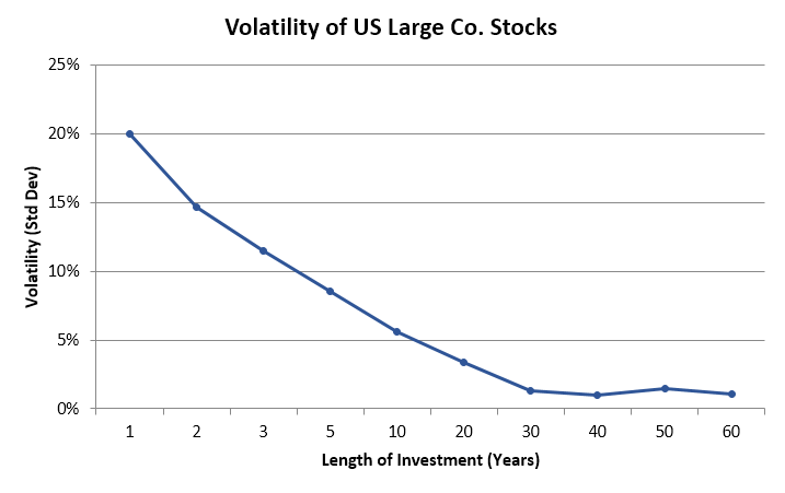
Source: Shiller website
Forecasting returns over short periods of time, say 1 or 2 years, would appear to be highly speculative, having more in common with gambling than making a serious estimate. Returns have been substantially more stable over longer periods of time (the implication being that they are possibly more predictable), with a standard deviation of less than 5% once the length of investment reached 20 years. Time, as it turns out, has been a fantastic means of reducing volatility. A ten year time horizon ends up somewhere in the middle–substantially less speculative, but not exactly a slam dunk either.
Start Simple
The most straightforward development of the expected return formulation for stocks starts with the Gordon equation (sometimes referred to as the dividend discount model or Gordon growth model). The formula is attributed to economist Myron Gordon, and serves as a method to value the price of a stock based on current dividend, D, dividend growth rate, g, and a discount rate/expected rate of return, k.6 The equation is similar to that used in a discounted cash flow analysis:
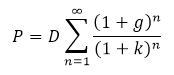
Solving for expected return, k, results in the following
k = D/P + g = Dividend Yield + Dividend Growth Rate
The calculation for expected return requires data on dividend yield and dividend growth rate, both of which can be derived from Robert Shiller’s Irrational Exuberance data.7 The real dividend growth rate, calculated over the entire 1871-2015 period, comes out to a 1.5% real rate of growth. (I should mention that all returns from this point forward will be real returns. This means using real dividend growth in the above calculation.) Dividend yield was taken as the end-of-year yield on US large company stocks from Ibbotson’s SBBI classic yearbook. The forecast and actual 10 year forward returns were computed every year starting in 1926 and running through 2005 for a total of 80 observations.
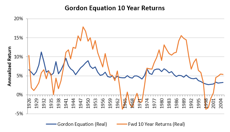
Here is a table of forecasting statistics associated with the chart above:
| 10 Year Forecasting Statistics | ||
| Gordon Forecast | Actual Returns | |
| Average | 5.59% | 6.82% |
| Standard Deviation | 1.68% | 5.57% |
| Minimum | 2.65% | -3.81% |
| Maximum | 11.22% | 17.90% |
| Range | 8.56% | 21.71% |
Use of this simple model has painted a rather rosy picture. There was no ten year period with a real annualized forecast of less than 2.65%. However, when compared to actual realized returns, the forecast suffered from the same problem as the CFOs–returns were expected to fall within a much tighter range than was realized. From this rather simple analysis it would appear that dividends, and the growth of dividends, fail to capture the full nature of 10 year forward stock returns.
The finding that forecasted returns using the Gordon equation are less volatile than realized returns is not a new idea. Stephen Foerster and Stephen Sapp of The University of Western Ontario came to a similar conclusion when they investigated the use of the dividend discount model to estimate the intrinsic value of the S&P 500.
Although many subsequent studies continue to find evidence in support of the predictive ability of dividends for equity returns, studies using longer time series of data bring the generalizability of these results into question – the predictive ability of the dividend ratio appears to be specific to a few time periods (e.g., Goyal and Welch (2003)). As a result, there is uncertainty regarding the importance one should give to dividends in the valuation of equities over time.8
An Improvement?
To improve the outlook Bogle, Bernstein and Research Affiliates all append an additional term to the Gordon equation. This term is meant to account for the change in price that, in theory, accompanies a change in dividend yield. As Bernstein explains in his book:
What if the dividend yield changes over time? For example, between 1926 and 1999, the dividend on the S&P 500 decreased from 5 percent to 1.1 percent. This annualizes out to a price increase from this fall in dividend of 2.1 percent per year. By contrast a rise in dividend implies a fall in price.4
As suggested by Bernstein in his book Rational Expectations, Shiller’s CAPE ratio has become the foremost tool for use in predicting the expected price change of US stocks.9 From 1881 through 2015, Shiller’s Cyclically Averaged Price-Earnings (CAPE) Ratio has averaged approximately 16.6. Using this information combined with the end-of-year CAPE one can formulate a “CAPE Mean Reversion” term that is annualized over ten years to estimate the annualized change in price:
![]()
Combining the Gordon equation with the mean reversion of the CAPE ratio produces a new expected returns equation:
k = Dividend Yield + Real Dividend Growth Rate + CAPE Mean Reversion
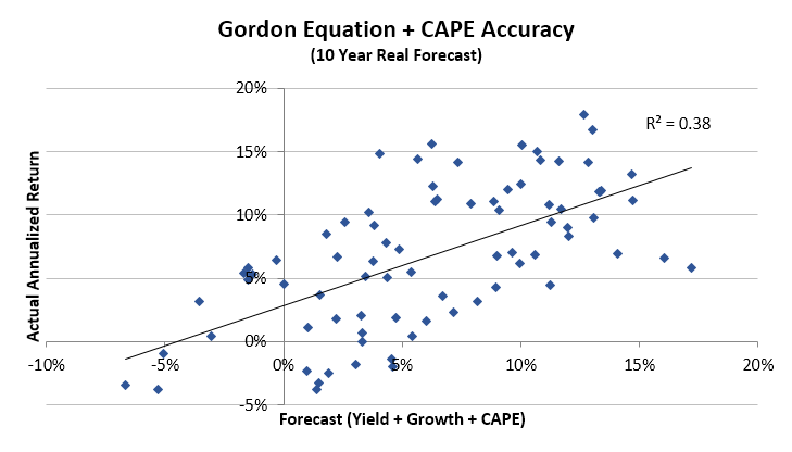
After running this updated model, a simple visual inspection shows that forecast returns now track actual returns a little better.
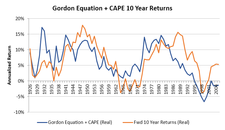
The statistics below confirm that the model now captures the broader range of possibilities:
| 10 Year Forecasting Statistics | ||
| Gordon+CAPE Forecast | Actual Returns | |
| Average | 6.23% | 6.82% |
| Standard Deviation | 5.44% | 5.57% |
| Minimum | -6.68% | -3.81% |
| Maximum | 17.17% | 17.90% |
| Range | 23.85% | 21.71% |
At first blush the above numbers look spectacular, especially compared to the original model without the mean reverting CAPE. A regression analysis also shows a reasonable trend:
The Perfect Solution?
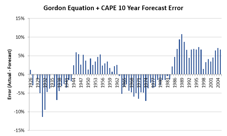
Don’t get too excited. Although the model has, collectively, captured the range of historic 10 year returns, it is still very much a blunt instrument. In any given 10 year period the error of this “improved model” has been huge. Since 1985 it has under-predicted actual 10 year annualized returns by an average of almost 6%. On two occasions the annualized error exceeded the actual return by more than 10% (1931 and 1989).
In a similar manner, Shiller’s own forecasting effort with the CAPE ratio wasn’t exactly accurate. When he first proposed using the CAPE ratio back in 1997 his comments read as follows:
Noting that the price-smoothed earnings ratio for January 1997 is a record 28, the regression illustrated in Exhibit 6 is predicting a decline of 0.5 in the log real stock price. In percentage terms, it is predicting that the real value of the market will be 40% lower in ten years than it is today. The corresponding forecast for the cumulative continuously compounded real stock return is -15% over ten years.10
From Shiller’s own data the real stock price in January 1997 was 1156.35, and by January 2007 it was 1689.35—46% higher than it was in 1997. While not incredibly accurate for the 10 year period, the forecast did warn that the market was overvalued, with the ensuing crash beginning in 2000 and extending into early 2003.
Being Reasonable
The major difference between expected returns and the market prediction du jour is that the former deals with the mechanics of asset valuation. It assumes a reversion to the mean without knowledge of when that reversion will occur. As the regression above shows, the forecast does have a relationship to the forward ten year returns, it just isn’t very accurate. On a practical level the formulations presented above require a strong dose of humility. Consider Rob Arnott’s comments from his Research Affiliates whitepaper:
It is very difficult, if not impossible, to create a model that results in perfect absolute forecasts, but if the model is internally consistent, the results will allow for relative comparison between asset classes, even if the estimated absolute returns prove to be inaccurate.5
My intention here was not to poke holes in mathematical models or attempt to come up with a better one. It was to highlight the realities of real world forecasting, which I believe has applications well beyond the world of finance. As the results above suggest, we live in a highly unpredictable world in which there is a very broad range of possible outcomes. This shouldn’t come as a surprise. Models aren’t bad. Historic probabilities aren’t bad. But they need to be used in a responsible manner. Their shortcomings should be understood and potential errors assessed. Reliance on models without acknowledging where they can and will go wrong is a recipe for disaster.
For those looking for more in-depth views of forecasting models, I recommend you check out Wes’s old post on the subject.
References
- Johnston, Michael. A Visual History of Market Crash Predictions. fundreference.com. July 16, 2015. http://fundreference.com/articles/2015/1000555/the-clowns-of-wall-street.
- Ben-David, Itzhak, John R. Graham and Campbell R. Harvey. Managerial Miscalibration. The Quarterly Journal of Economics. September 2013.
- Rekenthaler, John. JACK BOGLE: Get ready for a decade of 6% annual returns in the stock market. Business Insider. November 13, 2015. http://www.businessinsider.com/bogle-stocks-to-gain-about-6-over-the-next-decade-2015-11
- Bernstein, William. The Investor’s Manifesto. John Wiley & Sons, Inc. Hoboken, NJ. 2010. pp. 25-35.
- Capital Market Expectations. Research Affiliates white paper. https://www.researchaffiliates.com/Production%20content%20library/AA-Expected-Returns-Methodology.pdf
- Gordon, Myron J. The Investment, Financing, and Valuation of the Corporation. Martino Publishing. Mansfield Centre, CT. 2013. pp. 63-66.
- Shiller data
- Foerster, Stephen R. and Stephen G. Sapp. Dividends and Stock Valuation: A Study From the Nineteenth to the Twenty-First Century. University of Western Ontario. March 13, 2006. http://papers.ssrn.com/sol3/papers.cfm?abstract_id=890445
- Bernstein, William. Rational Expectations. 2014. pp. 36-39.
- Shiller, Robert J. and John Y. Campbell. Valuation Ratios and the Long-Run Stock Market Outlook. The Journal of Portfolio Management. Winter 1998. pp. 11-26. http://www.econ.yale.edu/~shiller/online/jpmalt.pdf

About the Author: Daniel Sotiroff
—
Important Disclosures
For informational and educational purposes only and should not be construed as specific investment, accounting, legal, or tax advice. Certain information is deemed to be reliable, but its accuracy and completeness cannot be guaranteed. Third party information may become outdated or otherwise superseded without notice. Neither the Securities and Exchange Commission (SEC) nor any other federal or state agency has approved, determined the accuracy, or confirmed the adequacy of this article.
The views and opinions expressed herein are those of the author and do not necessarily reflect the views of Alpha Architect, its affiliates or its employees. Our full disclosures are available here. Definitions of common statistics used in our analysis are available here (towards the bottom).
Join thousands of other readers and subscribe to our blog.