We can define popularity as the condition of being admired, sought after, well-known, and/or accepted. One would think popularity is a good thing. However, when it comes to investing, the research shows that along with popularity comes lower returns—results that sometimes conflict with traditional economic theory where risk and expected return should be positively related.
Consistent with traditional economic theory, investors dislike risk. Thus, riskier assets generally have higher returns.
Some examples:
- Riskier stocks have provided higher returns than safer bonds;
- riskier small stocks have provided higher returns than safer large stocks;
- riskier long-term bonds have provided higher returns than safer short-term bonds.
However, we have an anomaly in that riskier small growth stocks have underperformed safer large growth stocks, and they also underperformed even riskier small value stocks. What explains the underperformance?
One explanation for this and other anomalies, offered by Roger Ibbotson and Thomas Idzorek in their paper “Dimensions of Popularity,” which appeared in the 2014 special anniversary issue of the Journal of Portfolio Management, is that there are certain characteristics that make investments popular. That popularity induces investment, which in turn drives up prices and drives down returns. Conversely, there are securities with characteristics that make them unpopular with investors (for example, negative skewness and excess kurtosis, or fat left tails, which increases the risk of large losses)—they tend to avoid them, driving down their prices, and increasing their expected returns.
Behavioral finance has provided us with examples of investor preferences creating anomalies. For example, the poor performance of small-cap growth stocks (sometimes referred to as the “black hole of investing”) is explained by their popularity—individual investors have a preference for assets whose distribution of returns resembles that of a lottery ticket (positive skewness and excess kurtosis resulting in a large tail in the right-hand side of the distribution—the mean return is poor but there is a small chance of a very large return). It turns out that many kinds of securities with a low (or even negative) expected return, but with a small chance of a “jackpot” payout have poor risk-adjusted returns—not just small growth stocks. Others “jackpot” assets include deep out-of-the-money options, IPOs, penny stocks, and stocks in bankruptcy.
Another example of popularity relates to liquidity. Roger G. Ibbotson and Daniel Y.J. Kim—authors of the July 2014 study “Liquidity as an Investment Style” concluded that there’s an inverse relationship between returns and risk (in terms of volatility), with the low-liquidity portfolio (least popular stocks) having the highest return but the lowest risk.
The bottom line is that the field of behavioral finance has provided us with another insight into expected returns besides risk. Ibbotson and Idzorek explain:
The payoff [in the form of a premium] is not just for risk but also for anything investors find to be intrinsically unattractive, for example, less liquid, high taxability, difficult to diversify, high search costs, bad management, distress, and so on.
We see this play out in many ways. For example, Peter Lynch advised investors to “buy what you know.” This leads investors to buy stocks with which they are familiar. These stocks are likely to be large growth companies and stocks that are in the news most often. And it leads to the mistake I refer to as confusing the familiar with the safe. It can also be an explanation for the momentum effect. Stocks that have recently done either the best or the worst tend to be in the news. Investors jump on the “bandwagon” (buying yesterday’s winners and selling yesterday’s losers), generating momentum.
Another example relates to socially responsible investing or ESG (environmental, social, and governance) investing. The popularity of companies with favorable ESG rankings increases the demand for their stocks, driving prices higher. The reverse is true of “sin” stocks. Predictably, the result is that sin stocks outperform. For example, Harrison Hong and Marcin Kacperczyk, authors of the study “The Price of Sin: The Effects of Social Norms on Markets,” found that for the period from 1965 through 2006, a U.S. portfolio long sin stocks and short their comparables posted a return of 3.5 percent a year above their peers after adjusting for the Carhart four-factor (beta, size, value and momentum) model. As out-of-sample support, sin stocks in seven large European markets and Canada outperformed similar stocks by about 2.5 percent a year.
While acknowledging that there may be many ways to define popularity, in their paper, Ibbotson and Idzorek use turnover as one measure of popularity. They showed that stocks with the lowest turnover (least popular) had the highest returns and the lowest risk, and the relationship was monotonic as you moved across quartiles.
New Equilibrium Theory (NET)
In their 1984 paper, “The Demand for Capital Market Returns: A New Equilibrium Theory.” Roger Ibbotson, Roger G., Jeffrey, J. Diermeier, and Laurence B. Siegel proposed a new asset pricing theory that accounted for all the additions and subtractions for desired and undesired characteristics. In a just published book, “Popularity: A Bridge between Classical and Behavioral Finance,” Roger G. Ibbotson, Thomas M. Idzorek, Paul D. Kaplan, and James X. Xiong, crafted NET into a new popularity asset pricing model (PAPM) which combines elements of both classical and behavioral finance. The PAPM is based on the following pillars of economic theory.
- Subjectivism—The values of assets are not determined
solely by their inherent properties. Investor preferences play a major role in determining
value.
- Marginalism—Each investor constructs his or her portfolio so that the marginal contribution to utility of each asset is equal to the marginal cost of holding the asset—its price.
- Equilibrium— Asset prices are determined in markets so that all assets are willingly held.
The authors note that some aspects of popularity are systematic and quasi-permanent. Other aspects of popularity may be transitory or exist only as fads:
For example, liquidity is permanently popular, but on a relative basis during times of market distress, it is especially sought after. Society places a greater relative value (monetary or otherwise) on the more popular items.
Their popularity framework includes a generalization of a wide range of characteristics in classical finance and behavioral finance that influence how investors value securities. They classify these characteristics into two broad categories with two subcategories each:
Classical:
1. Risks: In classical finance, risk usually refers to fluctuations in asset values, but risk can be interpreted more broadly as any risks to which a rational investor would be averse.
2. Frictional: Examples include taxes, trading costs, and asset divisibility.
Behavioral:
1. Psychological: Investors consider these characteristics because of their psychological impact. For example, buying a company with a small carbon footprint might make an investor feel good.
2. Cognitive: Investors consider these factors or fail to accurately interpret such factors because of systematic cognitive errors. For example, investors may overvalue the importance of a company’s brand when evaluating its stock because they do not realize that the value of the brand is already embedded in the market price of the stock.
Summarizing, “assets are priced not only by their expected cash flows but also by the popularity of the other characteristics associated with the company or security. The less popular stocks have lower prices (relative to the expected discounted value of their cash flows), thus higher expected returns. The more popular stocks have higher prices and, therefore, lower expected returns. Popularity can be related to risk (an unpopular characteristic), and it can also be related to other rational preferences. But popularity can also be related to behavioral concepts.”
The following table presents the popularity-based explanations of premiums and anomalies:
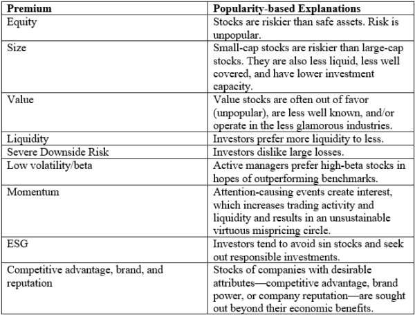
The authors then presented the evidence on each of the premiums.
Popular Company Characteristics
Although a single mutually agreed-upon best measure of a security’s popularity does not exist, the authors identified several previously unstudied characteristics that could serve as proxies for dimensions of popularity. These traits include the value of a brand, the degree to which a company is estimated to have a sustainable competitive advantage, and the reputation of the company. They used the following measures of these dimensions of popularity:
1. Interbrand’s annual “Best Global Brands” report. On an annual basis, Interbrand publishes a list of the 100 brands with the highest estimated “brand value.” They tested whether significant performance differences exist among the evolving top 100 brands.
2. Morningstar’s economic moat ratings. Morningstar’s equity analysts evaluate several factors related to a company’s relative sustainable competitive advantage (considered a moat to deter competition), including network effect, intangible assets, cost advantage, switching costs, and efficient scale. Based on this analysis, they classify each company as having (1) a wide moat, (2) a narrow moat, or (3) no moat. A sustainable competitive advantage is an example of a characteristic that investors would nearly uniformly agree is good.
3. Nielsen’s Harris Poll reputation quotient. The Harris Poll reputation quotient measures the reputations of companies in the United States in which consumers rate corporations by 20 attributes that are categorized into six dimensions, which ultimately form the reputation quotient. They believe the reputation quotient aligns well with characteristics that investors seek and thus can serve as a proxy for a dimension of popularity.
For each popularity measure, the authors considered four portfolios formed by dividing the universe of stocks into equally populated quartiles such that quartile 1 contains the most popular stocks and quartile 4 contains the least popular stocks. In terms of brand value, on an equal-weighted basis, over the period April 2000 through August 2017, as you moved from quartile 4 containing the stocks with the lowest brand value (BV)—the least popular stocks—to Quartile 1 containing the stocks with the highest BV—most popular stocks—the lower-BV quartiles monotonically outperformed the higher-BV quartiles. Q4 stocks returned 12.0 percent versus 5.9 percent for the Q1 stocks. The same monotonic relationship holds for the Sharpe ratio: Q4 had a significantly higher Sharpe ratio (0.71) than the other three quartiles (Q1 Sharpe ratio was 0.34). They also found no consistent relationship for standard deviation across the quartiles. Directionally, the results were similar when portfolios were formed on a cap-weighted basis.
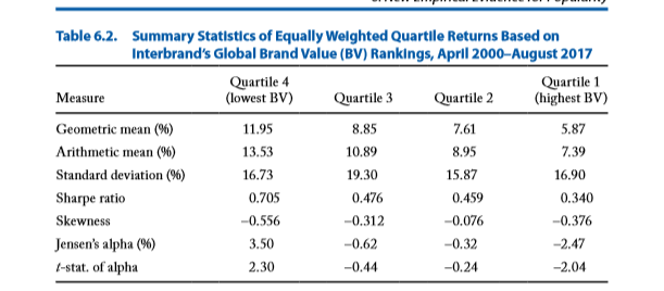
The results are hypothetical results and are NOT an indicator of future results and do NOT represent returns that any investor actually attained. Indexes are unmanaged and do not reflect management or trading fees, and one cannot invest directly in an index.
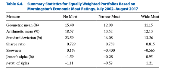
In terms of economic moat ratings, over the period July 2002 through August 2017, as we move from no-moat companies with, on average, the lowest sustainable competitive advantage (least popular companies) to the wide-moat companies with, on average, the highest sustainable competitive advantage (most popular companies), they found that the no-moat companies produced the most superior arithmetic and geometric mean returns. The additional return came, however, with more risk. On an equal-weighted basis, the annualized return/standard deviation of return/Sharpe for the no moat companies was 15.4%/23.6%/0.73 versus 11.2%/13.3%/0.82. Again, the results were directionally similar on a market-cap basis.
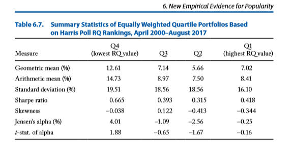
In terms of reputation, once again they found that as they moved from Q4 containing the stocks with the lowest reputation quotient (RQ)—most unpopular stocks—through the various quartiles to Q1 containing the stocks with the highest RQs—most popular stocks—the lower-RQ quartiles outperformed the higher-RQ quartiles. On an equal-weighted basis, the annualized returned/standard deviation/Sharpe ratio of Q4 companies was 12.6%/19.5%/0.67 versus 7.0%/16.1%/0.42 for companies in Q1. Again, the results were directionally similar on a market-cap basis.
The authors also looked at tail risk, which is unpopular.
Tail Risk
Over the period from January 1996 to August 2017, the stocks with the most tail risk (the least popular) outperformed the stocks with the least tail risk (the most popular). On an equal-weighted basis, the annualized returned/standard deviation/Sharpe ratio of Q4 (the most tail risk) companies was 12.2%/14.7%/0.74 versus 8.2%/14.8%/0.48 for companies in Q1. Again, the results were directionally similar on a market-cap basis.
The authors also looked at the aforementioned lottery stocks.
Lottery Stocks: Preference for Positive Skewness
Lottery-like stocks have a relatively small probability of a large payoff. From a popularity perspective, this strong preference for lottery-like stocks suggests that
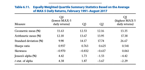
lottery-like stocks are popular. Using a measure called MAX-5 (the return on the five best days in the prior month), they found that moving from Q4, stocks with the lowest MAX-5 (least popular stocks), to Q1, stocks with the highest MAX-5 (most popular stocks), stocks with lower MAX-5 ratings monotonically produced superior Sharpe ratios. The monotonic increase in standard deviation is also clearly seen across the quartiles, and the highest MAX-5 quartile has the highest volatility. On an equal-weighted basis, over the period February 1991 through August 2017, the annualized returned/standard deviation/Sharpe ratio of Q4 (the most tail risk) companies was 11.6%/10.0%/0.94 versus 13.4%/26.7%/0.54 for companies in Q1. Note the dramatically lower Sharpe ratio for the stocks in Q1. When looking at cap-weighted results the picture is this time quite different. The annualized returned/standard deviation/Sharpe ratio of Q4 (the most tail risk) companies was 9.5%/11.3%/0.66 versus 8.4%/27.8%/0.36 for companies in Q1. Here we see the most popular stocks had the lowest returns and the most volatility.
Low Beta
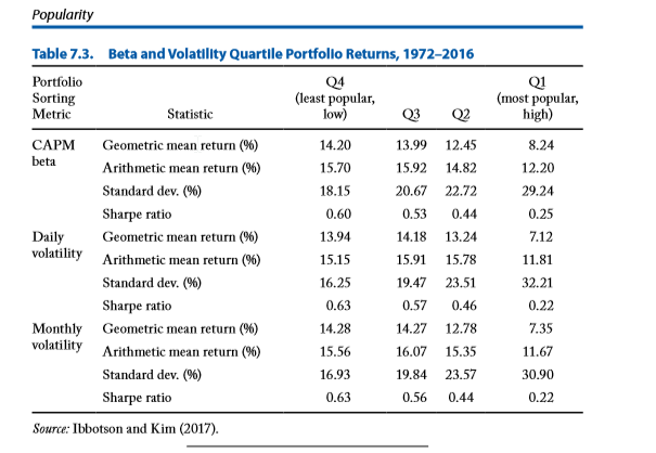
Over the period 1972 through 2016, the annualized returned/standard deviation/Sharpe ratio of Q4 (the least popular, low beta stocks) was 14.2%/18.2%/0.60 versus 8.2%/29.2%/0.25 for companies in Q1 (the most popular, high beta stocks). We see once again that popularity came at a price.
The results are hypothetical results and are NOT an indicator of future results and do NOT represent returns that any investor actually attained. Indexes are unmanaged and do not reflect management or trading fees, and one cannot invest directly in an index.
In their book, the authors also showed the well-documented evidence that smaller stocks and value stocks have provided higher returns than their large and growth counterparts.
Size
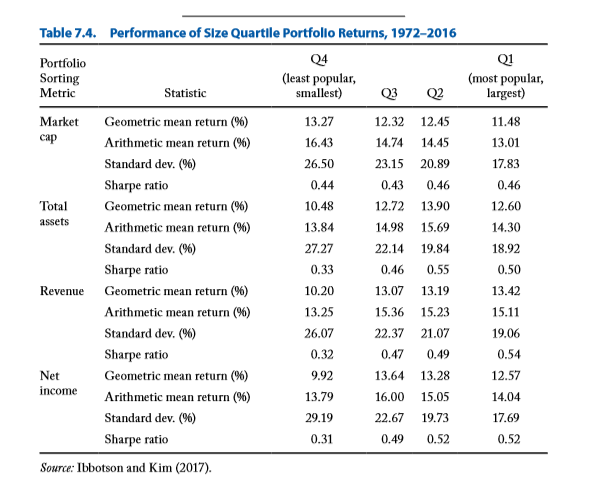
From 1972 through 2016, the stocks in Q4 (the smallest, least popular) stocks returned 13.3 percent a year versus the 11.5 percent return for the most popular stocks in Q1 (the largest stocks). Q4 stocks did exhibit much higher volatility, with the result being very similar Sharpe ratios (0.44 for Q4 stocks versus 0.46 for Q1 stocks).
Value
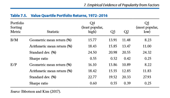
From 1972 through 2016, Q4 value stocks (the least popular) provided higher returns and higher risk-adjusted returns than did the more popular growth stocks. Using book-to-market as the measure of value, the annualized returned/standard deviation/Sharpe ratio of Q4 (the least popular, value stocks) was 15.8%/18.2%/0.60 versus 8.2%/24.3%/0.25 for companies in Q1 (the most popular, growth stocks). Using price-to-earnings as the measure of value, the annualized returned/standard deviation/Sharpe ratio of Q4 (the least popular, value stocks) was 16.1%/22.8%/0.60 versus 8.2%/27.9%/0.25 for companies in Q1 (the most popular, growth stocks).
Liquidity
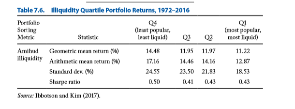
They defined liquidity as the absolute value of the daily return divided by the daily dollar value of shares traded, averaged over the course of the selection year. From 1972 through 2016, the annualized returned/standard deviation/Sharpe ratio of Q4 (the least popular, most illiquid stocks) was 14.5%/24.6%/0.50 versus 11.3%/18.5%/0.43. for companies in Q1 (the most popular, most liquid stocks). Q4 outperformed Q1 by a wide margin. This result is consistent with risk-based explanations because liquidity is always desired by some segments of the market, and those investors are willing to pay for it (accept lower returns).
Momentum
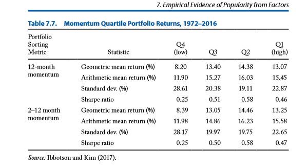
From 1972 through 2016, using the last 12 month’s returns to define momentum, the annualized returned/standard deviation/Sharpe ratio of Q4 (the least popular, lowest momentum stocks stocks) was 8.2%/28.6%/0.25 versus 13.1%/22.9%/0.46% for companies in Q1 (the most popular, highest momentum stocks). The results were similar when using the common measure of months t-2 and t-12 (omitting the most recent month). While popularity explains returns, momentum is an exception to the cross-sectional results we have seen so far with the most popular stocks outperforming. With that said, that popularity leads to higher valuations. The result is that momentum leads to the well-documented phenomenon of reversal in the return to momentum stocks over the longer term.
The authors did examine three other metrics that could be based on popularity: total assets (the larger companies being more popular); net income (more profitable companies being more popular); and revenue (the companies with higher sales being more popular). In these three cases the least popular companies did not outperform.
The Curse of Popularity
We see that all but the cases of the three exceptions mentioned above (and momentum, which is an anomaly for all models) the least popular stocks outperformed the most popular stocks. Regarding the three exceptions, the authors noted: “We believe they are almost never viewed in isolation and they are almost never the sole reason that an investment decision is made. Therefore, we do not interpret these results as definitive evidence against the popularity framework.” And, I’m not aware of any funds that use those metrics as screens to determine their eligible universe. Nor are they considered to be factors with explanatory power in the literature.
Summarizing, by including risk aversion and popularity preferences, the PAPM provides a bridge between traditional finance theory and behavioral explanations for pricing anomalies. Popularity preferences can be either rational (for example, a preference for ESG investments) or irrational, as in behavioral economics. These preferences are priced according to the aggregate demand for each of the characteristics.
The expected return of each security is determined by its risk and popularity characteristics.
At the very least, investors who express their preferences for stocks should be aware that those preferences can lead to below market returns. Being aware that preferences can reduce expected returns can help investors make rational choices about those preferences.
So, what’s popular today? In the next section we’ll take a look at two strategies that have become popular in recent years, low beta/low volatility and quality.
Popularity Case Studies: Low Beta and Quality
In our last selection we discussed what could be called the “curse of popularity”—with popular stocks producing lower returns than unpopular ones. Today, we’ll examine two strategies that have become popular based on the publication of research that has found that low beta/low volatility stocks have outperformed as have high quality stocks. For further reading on the low volatility/ low beta anomaly check out my earlier article here.
The superior performance of low-volatility stocks was first documented in the literature in the 1970s—by Fischer Black in 1972, among others—even before the size and value premiums were “discovered.” The low-volatility anomaly has been shown to exist in equity markets around the world. Interestingly, this finding is true not only for
Low beta investing has become particularly popular after the bear market of 2008. The largest low-beta fund is the and the iShares Edge MSCI Min Vol USA ETF (USMV) which, according to Morningstar, as of this writing (February 11, 2019), had almost $22 billion of assets under management. To see if the popularity of the fund has impacted its expected return we’ll examine various valuation metrics of the fund compared to those of the Schwab U.S. Broad Market ETF™ (SCHB). Data is from Morningstar.

The results are hypothetical results and are NOT an indicator of future results and do NOT represent returns that any investor actually attained. Indexes are unmanaged and do not reflect management or trading fees, and one cannot invest directly in an index.
No matter how which metric we use, USMV has higher valuations—it’s more growthy than the market. Thus, it has lower expected returns than the market. Consider the following. In his 2012 paper, “Enhancing a Low-Volatility Strategy is Particularly Helpful When Generic Low Volatility is Expensive,” Pim van Vliet found that while, on average, low-volatility strategies tend to have exposure to the value factor, that exposure is time-varying. The low-volatility factor spends about 62 percent of the time in a value regime and 38 percent of the time in a growth regime. The regime-shifting behavior affects the performance of low-volatility strategies. When low-volatility stocks have value exposure, they, on average, outperformed the market by 2.0 percent. However, when low-volatility stocks have growth exposure, they have underperformed by 1.4 percent, on average. In other words, the performance of low beta strategies is regime dependent. The bottom is that what low volatility strategies are predicting today is low volatility in the future, along with lower expected returns.
Let’s turn now to a look at quality.
The Quality Factor
High-quality companies have the following traits: low earnings volatility, high margins, high asset turnover (indicating efficient use of assets), low financial leverage, low operating leverage (indicating a strong balance sheet and low macroeconomic risk), and low stock-specific risk (volatility that is unexplained by macroeconomic activity). Companies with these attributes historically have provided higher returns, especially in down markets. In particular, high-quality stocks that are profitable, stable, growing, and have a high payout ratio outperform low-quality stocks with the opposite characteristics.
Studies such as “The Excess Returns of ‘Quality’ Stocks: A Behavioral Anomaly,” and “Quality Investing – Industry versus Academic Definitions” have found that quality companies historically have provided higher returns, especially in down markets. In particular, high-quality stocks that are profitable, stable, growing, and have a high payout ratio outperform low-quality stocks with the opposite characteristics. From 1927 through 2018 the quality factor (QMJ) has provided a premium of 4.5 percent. (Data from AQR).

The results are hypothetical results and are NOT an indicator of future results and do NOT represent returns that any investor actually attained. Indexes are unmanaged and do not reflect management or trading fees, and one cannot invest directly in an index.
The publication of the research findings led to the development of investment products that focused on this factor, and its popularity soared. As of February 11, 2019, the iShares Edge MSCI USA Quality Factor ETF (QUAL) had $9.3 billion of assets under management. To see if the popularity of the fund has impacted its expected return we’ll examine various valuation metrics of the fund compared to those of the Schwab U.S. Broad Market ETF™ (SCHB). Data is from Morningstar as of February 7, 2019.
Again, we see how investors preference for the quality characteristic has impacted valuations, with quality stocks trading at higher valuations than the market, and dramatically higher in the case of book value (74 percent higher) and cash flow (34 percent higher). Since valuations are the best predictor we have of future returns, investors should at least consider them when making investment decisions.
As we discussed in my prior post, contrarian investing, buying the unpopular, has tended to produce superior results. Keep this in mind as you consider your asset allocation. Valuations do matter.
About the Author: Larry Swedroe
—
Important Disclosures
For informational and educational purposes only and should not be construed as specific investment, accounting, legal, or tax advice. Certain information is deemed to be reliable, but its accuracy and completeness cannot be guaranteed. Third party information may become outdated or otherwise superseded without notice. Neither the Securities and Exchange Commission (SEC) nor any other federal or state agency has approved, determined the accuracy, or confirmed the adequacy of this article.
The views and opinions expressed herein are those of the author and do not necessarily reflect the views of Alpha Architect, its affiliates or its employees. Our full disclosures are available here. Definitions of common statistics used in our analysis are available here (towards the bottom).
Join thousands of other readers and subscribe to our blog.

