Quantitative factor portfolios generally use historical company fundamental data in portfolio construction. The key assumption behind this approach is that past fundamentals proxy for elements of risk and/or systematic mispricing. However, what if we could forecast fundamentals, with a small margin of error, and compare that with market expectations? Intuitively, this seems like a more promising approach. I explore this concept using best practices from the science of forecasting and machine learning techniques, namely Random Forests and Gradient Boosting. The goal of this research is to build a value composite model based on forecasted fundamentals to price and see how this works relative to the “old” method of using historical fundamentals to price.
My approach is as follows:
- I use the in-sample data to train the models to predict forward-looking earnings, free cash flow, EBITDA, and Net Operating Profit After Taxes.
- I use these forecasts to build a value portfolio that seeks to improve upon traditional, less sophisticated value approaches.
Bottom line?
The combined value portfolio out of sample did not produce statistically significant outperformance versus the equal weight portfolio (as a comparison to the long-only value composite) or versus cash (for the long/short portfolio).(1)
Background
Forecasting as a science has developed over the past decades with the use of standard statistical techniques, such as a multiple linear regression, to more advanced machine learning techniques.
Some of the best practices or ideas evidenced by research are as follows:
- Crowds can often arrive at a superior and more robust estimate than the best individual forecast under the right circumstances
- Using an ensemble of methods and approaches is often superior to a single approach
- Start with the base case (outside view) and work into the inside view (the nuances of the specific case)
With investing in equities there has been a prime focus on earnings (net income) projections as a proxy for sustainable company cash flow, which is the core input in a discounted cash flow valuation (DCF) for company valuation. In the quantitative investment domain, the data used for portfolio construction has primarily been actual historical data (e.g. Fama & French and AQR) to build portfolios based on specific metrics, such as the most well-known Market Value/Book Value ratio for the value factor.
On the discretionary side of asset management there has been more of a focus on the anticipated future of the economy and company profits, with the prize going to the superior analyst who can forecast better than the rest.
A natural curiosity: What if we combined the best practices of forecasting and machine learning, and then created a quantitative equity portfolio of the companies with the best forecasted earnings in relation to their current asset price?
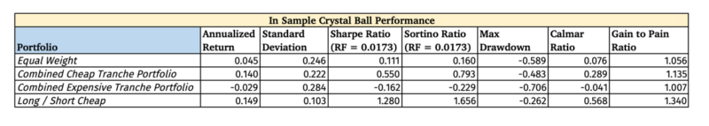
The Crystal Ball Portfolio
What is the portfolio performance if one could know in advance the next 12-month company fundamentals?(2)
I constructed this ideal Crystal Ball portfolio in the same way as the Random Forest model.
The Cheap portfolio is the cheapest 50% of stocks and the Expensive portfolio is the bottom 50% of stocks based on a composite valuation score from the following four factors:
- Price to 12 months forward 12 month trailing Free Cash Flow
- Price to 12 months forward 12 month trailing earnings
- 12 months forward 12-month trailing Return on Invested Capital
- Enterprise Value to 12 months forward 12 month trailing EBITDA
Each factor is winsorized at the 90% level to prevent the undue influence of outliers.
Next the factor values are given a Z score, and the final Valuations score is the sum of the four Z scores.
The portfolio has 4 tranches that each rebalance annually but individual tranches rebalance on subsequent quarter periods to minimize timing luck (Hoffstein, 2019). Tranches trade 3 months after the earnings date, to eliminate look-ahead bias, but is irrelevant in this example. For example, tranche 1 would trade the data from Q3 2000 at the end of Q4, since there is generally a one to three-month lag in earnings reports.
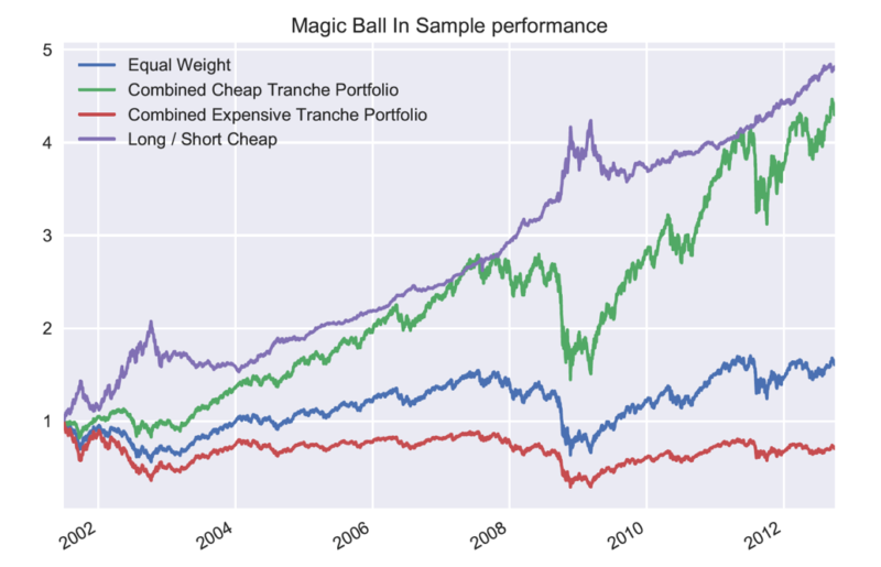
Below is the in-sample Crystal Ball Portfolios by Decile, where you can see the great risk and return differences. For obvious reasons, the portfolio Z scores were not winsorized in the below decile data.
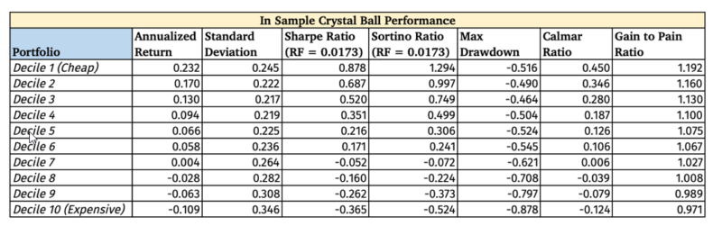
As to be expected, there is a high performance dispersion between deciles, and a mouth-watering Long/Short Sharpe Ratio of 1.28. But the results are designed to be unrealistic.
The main take away is that if we can reliably forecast the future fundamentals we can construct high return to risk portfolios.
Relevant Literature
Tetlock and Gardner (2016) have gleaned principles of superior forecasters. Superior forecasters start with a focus on the base case, or outside view (Kahneman (2015)), which is how a situation historically has transpired. After a reliable base case estimate is derived, then the unique details of the present situation are factored in to adjust the base case probability. Start with the historical pattern and adjust for the present. (related to Bayesian inference, discussed here with an application to investing.)
According to Surowiecki (2014), in order for crowds to have wisdom beyond any individual participant, they need to have the following characteristics:
- Independent
- Diversified
- Decentralized
- Have a pricing or voting mechanism as a way to aggregate information
For the above to lead to a good estimate from the crowd, the errors must be random and not systematically biased. This can often be untrue for asset markets because of the bias against short selling (potentially a non-issue for the futures market) and during bubbles/crashes the errors are biased towards the bull or bear case.
Tetlock and Gardner (2016) mention that superior forecasters know when there is madness of the crowds as well as wisdom of the crowds.
Machine Learning for Future Company Fundamentals
Alberg and Lipton (2017) used a deep neural network to form portfolios based on forecasted future fundamentals and saw a 2.7% annualized alpha vs. a standard factor based portfolio. They used data from Compustat starting in 1970, which provided a far greater number of data points to train their machine learning model vs. Sharadar’s data that starts in 1999. Shiller (1980) mentioned how stocks move more than they should if the price of a stock was the best predictor of future dividends. Thus, there is a high noise-to-signal ratio for individual stock prices, but I assume there is a lower noise-to-signal ratio with company fundamentals due to the greater stability and lower variance of fundamental data from one quarter to the next. Moreover, with the large number of different types of agents in the stock market with different motivations it will be hard to tease out singular causes behind stock price movements.
There has been research conducted using machine learning techniques around portfolio construction and risk assessment (see De Prado, 2016 and Zatloukal, 2019), but not much on creating portfolios based on forecasted company fundamentals.
Random Forests — An Introduction
Random Forests is a supervised machine learning technique that uses a composite of decision trees to make a forecast.(3) The Random Forests can be used as a classification (e.g. will the price of the stock go up or down) and as a regression function (i.e. what will the earnings be next quarter?) The researcher chooses the hyper parameters that the Random Forests uses to create the decision trees. The main hyper parameters for Random Forests are the number of Forests to create, the maximum depth of each forest, and the number of random features to use in each forest for splitting the decision tree.
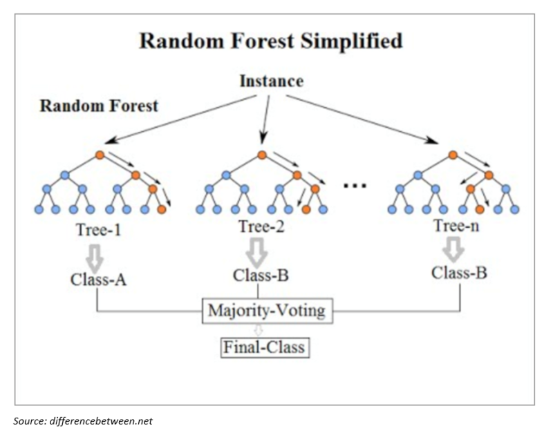
Random Forests utilize the wisdom of crowds, namely that “a large number of relatively uncorrelated models (trees) operating as a committee will outperform any of the individual constituent models” (Yiu, 2019). Uncorrelated models combined can do well since “the trees protect each other from their individual errors (as long as they don’t constantly all err in the same direction)” (Yiu, 2019). The uncorrelated errors can cancel each other out and allow the signal to emerge.
Random Forests use Bootstrap Aggregation, where a random sample (with replacement) of the training data is used to construct a decision tree. Moreover, a random set of features is used to split the decision tree. This added randomness aims to minimize variance and overfitting (Yiu, 2019). The final decision tree is an average of all the created forests (Burkov, 2019).
The Random Forest Regressor Function from Python’s Scikit-Learn Machine Learning package was used for the research with the following parameters:
- n_estimators = 1000
- random_state = 42
- criterion = “mse”
- max_depth = None
- max_features = 16 (1/3 of feature set)
Data
US Equity price and fundamental data is from Sharadar, and has all listed and delisted US traded equities from 1999 up until the present.
The in-sample data is from January 1st 1999 until the 31st of December 2012, of which the most recent 25% of the in-sample data is used as a validation set.
The out-of-sample data is from January 1st, 2013 to September 30th 2019.
Transactions costs, taxes, and slippage are ignored.
Quantitative Process and Rationale (Methodology)
The overall objective is to predict the next 12 months of earnings, net operating profit after taxes (NOPAT, used in ROIC calculation), free cash flow, and earnings before interest, tax, depreciation, and amortization (EBITDA) for US-traded companies using a Random Forests model. Assuming the model is accurate, rank stocks based on current price to forecasted fundamentals and invest in the cheapest 50% (long only) and/or short the most expensive (50%).
I constrained the data set to only US domiciled equities (listed and delisted). I isolated each equity sector for training the Random Forest model with the assumption that a more homogenous group of companies, i.e. a specific sector, would have more easily discernable drivers to sales and earnings.
My features are broken down into two categories: Economic and Company Specific Fundamentals.
The economic features were chosen to capture the overall economic environment, with many shown to have predictive power over future economic contractions, such as the yield curve (Estrella, 1996), and would hopefully reveal whether the economic environment was conducive to company profits.
Economic Features (Source: St. Louis FRED and Institute for Supply Chain Management):
- Consumer Price Inflation (CPI)
- Core CPI
- West Texas Intermediate Oil Price
- Price of Gold
- 10 Year Treasury Yield
- 3 Month Treasury Yield
- 10 Year – 3 Month Yield spread
- 3 Month LIBOR (USD)
- High Yield Option Adjusted Spread
- Investment Grade A Option Adjusted Spread
- High Yield OAS – Inv. Grade A OAS (Credit spread)
- Dollar Index
- Unemployment Rate
- Real Personal Consumption
- Building Permits
- Wilshire 5000 Index
- ISM Manufacturing PMI Index
- TED Spread
Company Fundamentals (source: Sharadar, calculations my own):
- Revenue
- Capital Expenditure
- Debt to Equity
- Earnings Before Income Tax, Depreciation, and Amortization (EBITDA)
- Operating Income
- Tax Expense
- Gross Profit
- Research and Development
- Selling and General Administration Expense
- Interest Expense
- Return on Invested Capital
- Return on Equity
- Enterprise Valued to EBITDA
- Current Debt
- Non-Current Debt
- Deferred Revenue
- Depreciation and Amortization
- Inventory
- Asset Turnover
- Working Capital
- Capital Expenditures to Sales
- Year on Year Revenue Growth
- Year on Year Net Income Growth
- Year on Year Net Cash Flow from Operations Growth
- Sector Year on Year Net Income Average
- Ratio of Company vs. Sector Year on Year Net Income Growth
- This feature was chosen to measure the base case growth for the industry with the assumption if the company was doing exceptionally well there was likely a reversion to the mean potentially in the future
- Sector Year on Year Revenue Average
- Ratio of Company vs. Sector Year on Year Revenue Growth
- Earnings Accrual Ratio
I included all companies that had a market capitalization of $1 billion or more based on the previous quarter in order to minimize liquidity issues in trade execution.
After the Random Forests model was trained, the model predicted the forward 12 month earnings, EBITDA, NOPAT, and free cash flow for each company. Note that there was a Random Forests model for each of the 4 factors and for each sector, resulting in 44 Random Forests models. From there, the portfolio would be constructed by going Long the cheapest 50% of companies (lower price to forecasted earnings, for example) and short the most expensive 50% of companies.
The four fundamental factors:
- Return on Invested Capital
- Price to Earnings
- Price to Free Cash Flow
- Enterprise Value to Earnings Before Interest, Tax, Depreciation, and Amortization (EBITDA)
Each factor is winsorized at the 90% level to prevent the undue influence of outliers
Next the factor values are given a Z score, and the final Valuations score is the sum of the four Z scores.
The portfolio has 4 tranches that each rebalance annually but start on subsequent quarter periods. I have utilized the staggered portfolio tranche composition to avoid timing luck in the rebalancing dates. The tranches trade 3 months after the earnings date to eliminate look-ahead bias. For example, tranche 1 would trade the data from Q3 2000 at the end of Q4, since there is generally a one to three month lag in company fundamental reports. The combined portfolio only uses the dates when all 4 tranches are active and invested.
Each Sector would have their unique value portfolio. Then all 11 sector portfolios are combined equal weight to create the overall Value portfolio.
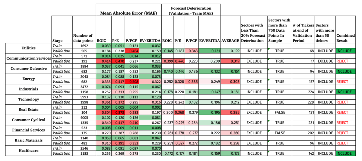
Descriptive Statistics
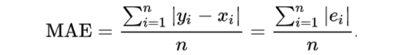
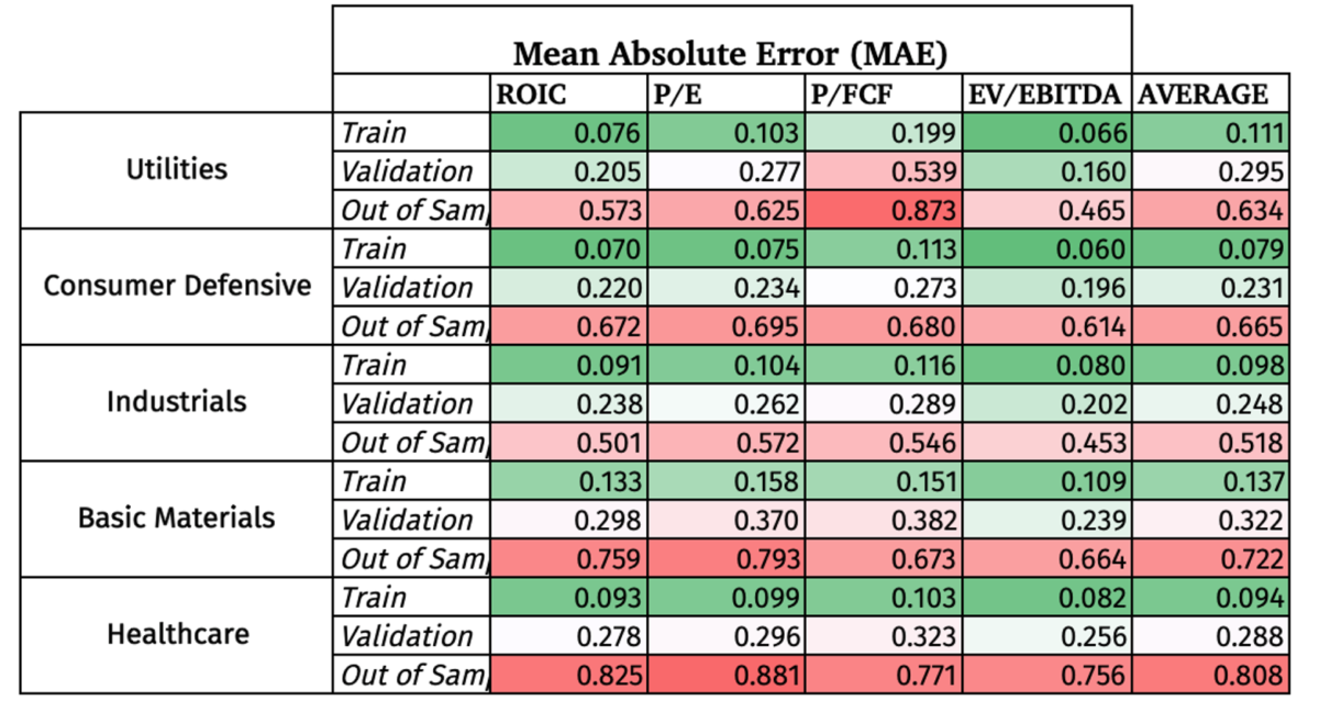
The Mean Absolute Error measures the absolute percentage difference between the Random Forest forecast and the actual data, with lower being better. It is a common metric to test the accuracy of a machine learning regression model.
The in sample has the lowest MAE by design, and the validation set increased slightly. But the big surprise is how high the MAE was in the Out of Sample data. I have colored coded the results to make it easier to see the contrast.

After testing the strategy in-sample (train vs. validation), the 11 sectors were narrowed down to those sectors that meet all three criteria:
- At least 50 companies at the end of the in-sample time period
- More than 750 data points to train the model
- Less than 20% deterioration in the MAE from in-sample to validation.
This resulted in choosing only 5 sectors, namely, Utilities, Consumer Defensive, Industrials, Basic Materials, and Healthcare.
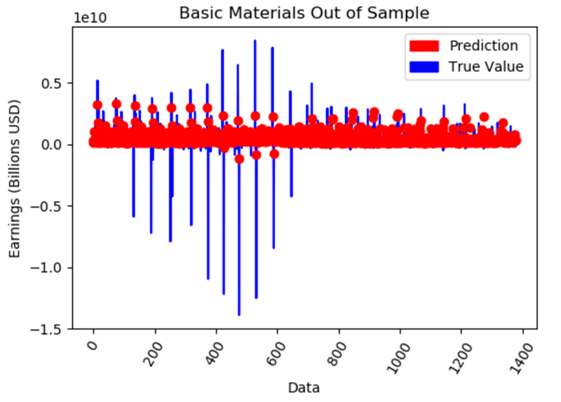
Besides the obvious deterioration in the MAE out of sample, the model did the best job at accurately forecasting EBITDA compared to the other 3 metrics, but with still a high MAE.
Here is an example of what is looks like to have such a high MAE out of Sample.
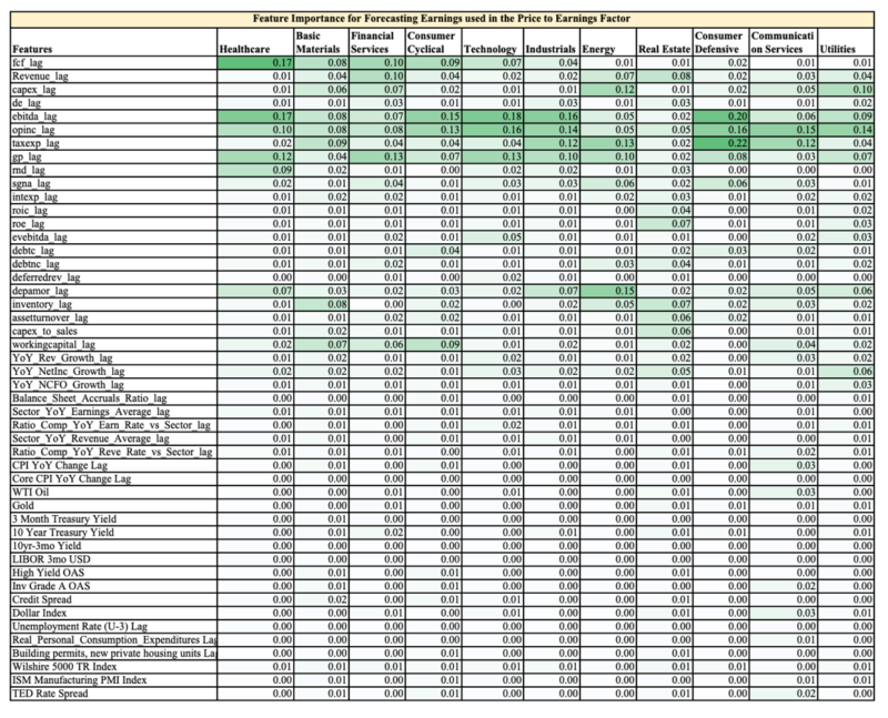
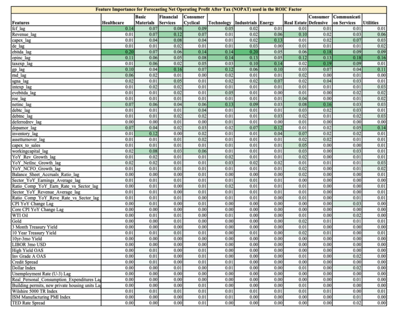
Below is a table showing the relative feature importance (0.17 = 17% out of 100%) in the final Random Forests Model for each sector, highlighted to provide easier digestion of the numbers.
The first 30 features are company fundamental data and the rest are macro-economic data.
You can easily see two observations:
- The company fundamental data is far more important than the overall macro environment when it comes to forecasting future earnings
- Each sector has different ranking of feature importance, hence the value of training the Random Forests models on each sector vs. on the overall market.
As an aside, a discretionary analyst could use this feature importance to help them focus on the most influential variables when forecasting company fundamentals.
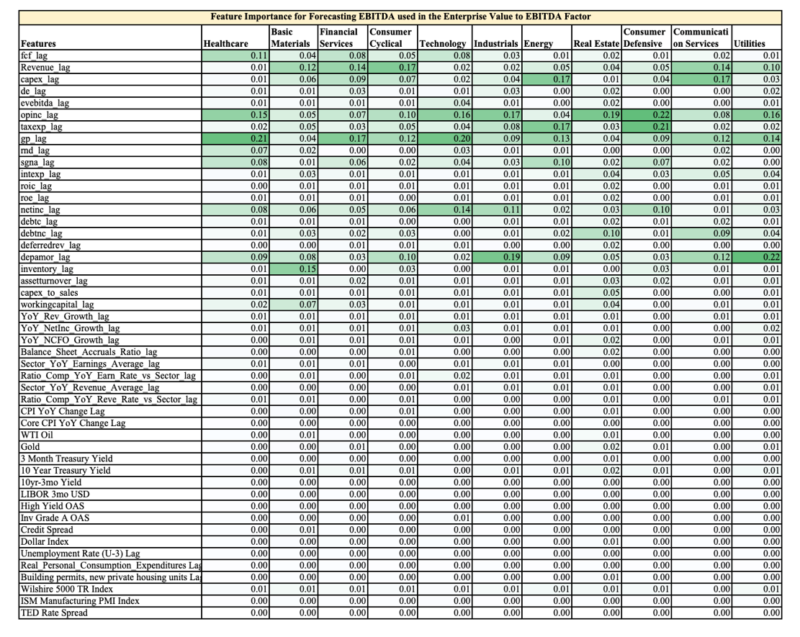
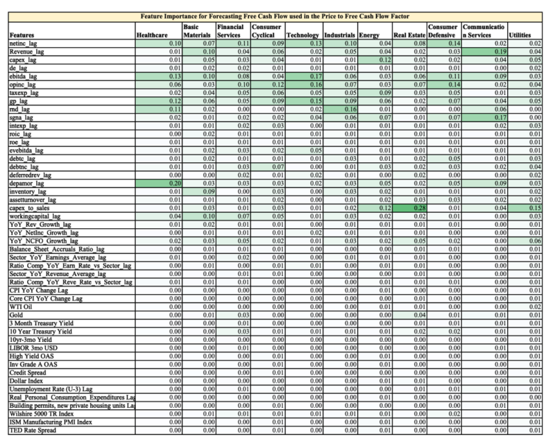
The appendix has the feature importance for Price to Free Cash Flow, Enterprise Value to EBITDA, and ROIC.
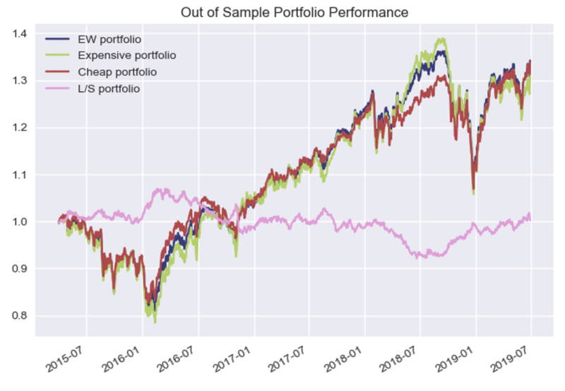
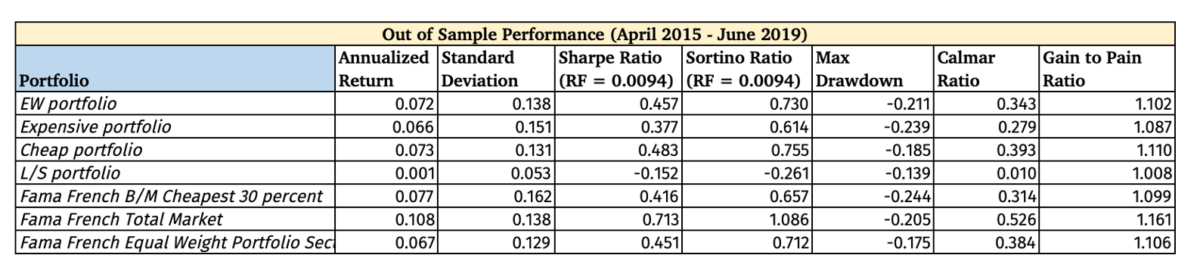
Nothing remarkable stands out from the performance chart above, except the slight outperformance and underperformance of the Long-Short portfolio in 2016 and 2018 respectively.
Note that even though the out of sample fundamental start in Q1 of 2013, it takes 5 quarters to get Year on Year feature data, 1 quarter of lag time in trade execution, and 3 quarters to have data for all 4 tranches, thus the first combined portfolio data starts in April 2015 (Q2).
Now vs. Fama French Total Market Data:
- B/M Cheapest – the cheapest 30% of USA traded companies based on Book to Market
- Total Market – Market Cap weighted total market value
- Equal Weight Portfolio Sectors – 20% in each of the 5 sectors used in Out of Sample Portfolio test to try to compare apples to apples
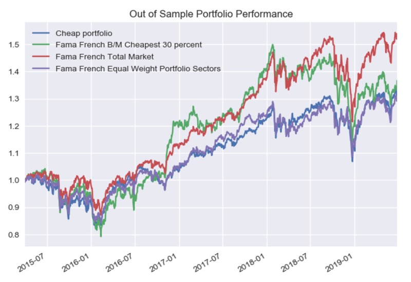
The large performance discrepancy above for the Total Market index is driven in part by the allocation to Technology, which was not included in the RF model.
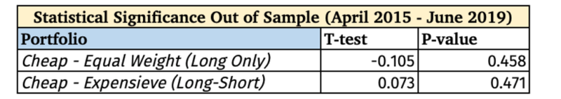
Statistical Significance of Findings
The Long only and Long-Short portfolio did not generate a high t-stat to make it statistically significant at the 5% level.
Analysis of Findings
Why was there such lackluster performance in the Random Forest’s ability to forecast future fundamentals? Looking at the R^2 score (table below), shows that the Random Forests Model, going from the train to validation to test data set, explains less and less of the actual future fundamental values (i.e. actual earnings) which is to be expected to some extent.

Moreover, as shown previously, the Mean Absolute Error Percentage increases significantly from the train to validation to the test data.
In essence, the model did not do a good job forecasting future fundamentals.
This can mean a few things:
- The Random Forests Model with this data set, regardless of any additional features added to the feature set, could not predict accurately enough the future company fundamentals to create alpha
- Another machine learning model could have produced alpha with this dataset (we will look at Gradient Boosting later in the post).
- There are qualitative (i.e. How strong is the moat of the company?) or hard to quantify factors that determine the future fundamentals of a company that were not a part of the model
- A systematic and quantitative machine learning model won’t work across a sector and each company will need more customizable forecasts.
Mean Absolute Error for Other Models
How do other ML models work in general vs. Random Forests?
Below are three other models combined with a simple linear regression model. The following ML models and their corresponding Scikit-learn function:
- Random Forests – sklearn.ensemble.RandomForestRegressor
- Gradient Boosting – sklearn.ensemble.GradientBoostingRegressor
- Support Vector Machines – sklearn.svm (data normalized)
- Neural Network – sklearn.neural_network.MLPRegressor (data normalized)
- Linear Regression – sklearn.linear_model.LinearRegression
I kept the hyper parameters in accordance with their default values and did not tune the hyper parameters. Moreover, I used all companies and sectors with a market cap of $1 billion or more and did not train a unique model on each sector.
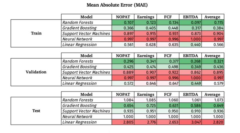
A few observations:
- EBITDA continues to be the easiest to predict out of sample (test) compared to the 3 other fundamental factors, which makes sense since it is the “highest” on the income statement and requires the least number of steps to arrive at from revenue. I would postulate that revenue would be the easiest to predict.
- The Linear Regression model had the greatest over fit, followed by the Random Forests model when looking at how the train, validation, and test MAE changed
- It is interesting to see that the Support Vector Machines (SVM) had roughly the same MAE for train, validation, and test, although it was quite high around .90
- Gradient Boosting substantially beat the Random Forests model out of sample.
- The Neural Network Model was essentially a random guess and added no value at all with an approximate 1.00 MAE even with Train and Validation sets
- The general Random Forest model, which trained and tested on all companies had an average MAE of 1.073 out of sample, but had an average MAE of .6694 on the five sectors (Utilities, Consumer Defensive, Industrials, Basic Materials, Healthcare) on average across all four fundamental factors out of sample. By implication, if the Gradient Boosting model was trained on each sector by themselves and their hyper parameters were tuned using the validation data set, it likely the MAE out of sample for the Gradient Boosting model would be even lower.
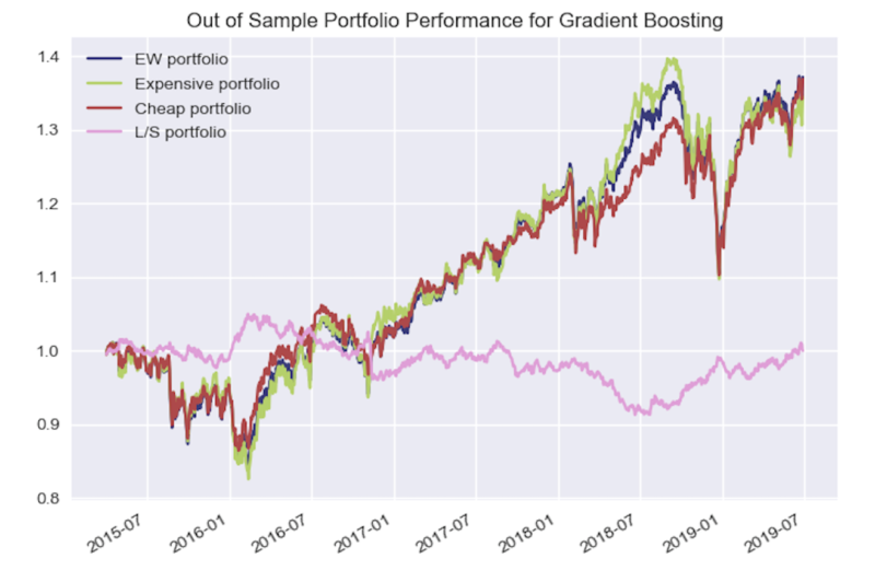
Hindsight “Out of Sample” Portfolio Performance
While committing a research felony by testing more than once on the out of sample dataset, out of curiosity, how would the Gradient Boosted (GB) model have work in portfolio construction? The GB model obviously did a better job in general on out of sample prediction. If we come to find that the GB model generates alpha we would need to be very stringent by using a Deflated Sharpe Ratio (Bailey, 2014) or very high statistical significance level (i.e. 99% or higher) to tease out luck.
Both Random Forests and Gradient Boosting are composed of decision trees.
The two main differences (Glen, 2019) are as follows:
- How trees are built: random forests build each tree independently while gradient boosting builds one tree at a time. This additive model (ensemble) works in a forward stage-wise manner, introducing a weak learner to improve the shortcomings of existing weak learners.
- Combining results: random forests combine results at the end of the process (by averaging or “majority rules”) while gradient boosting combines results along the way.
The Gradient Boosting Regressor Function from Python’s Scikit-Learn Machine Learning package was used for the research with the following parameters tuned after cross-validation:
- n_estimators = 3000
- random_state = 42
- min_samples_split = 2
- max_depth = 4
- learning_rate= .01
- loss = ‘ls’
Below we have the same MAE format as with the Random Forests model, but this time Basic Materials didn’t make the cut off.
Below are the MAE percentages for all five sectors included in the Out of Sample Random Forests Model for comparison:
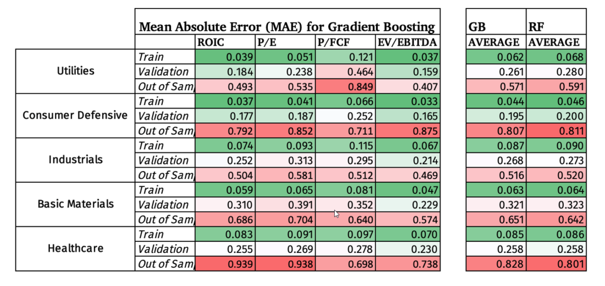
We can see that the Gradient Boosting model did not produce, on average, superior predictions compared to the Random Forests model, which is to some extent surprising since the general GB model did significantly better out of sample than the RF model. However, since GB and RF are both ensemble models that use decision trees it is understandable that they would create very similar results.
We see below a very similar and unimpressive performance for the GB model as with the RF model.

Further Research and Conclusion
In conclusion, the Random Forests and Gradient Boosting machine learning models did not produce statistically significant outperformance, which is primarily driven by their high Mean Absolute Error Percentages. In other words, the machine learning models had high variance and weren’t very accurate in their ability to predict future company fundamental values.
A good comparison would be to see if Wall Street Analysts on average do a better job at predicting future fundamentals vs. the Random Forests model, which could be done using Zach’s Consensus Earnings Estimate History Database. Moreover, I would expect the model to have performed better out of sample if I had access to the Compustat and CRSP data which would extend the data by around 37 years (back to 1963). With access to those databases you could use deep learning and other unsupervised techniques which require larger datasets than the one I had access to with Sharadar.
Another interesting concept to explore further would be around the idea of the range of accuracy needed in forecasting fundamentals to achieve alpha. Specifically, what level of Mean Absolute Error Percentage does a manager or analyst need when forecasting earnings, for example, to achieve alpha? Could an investor beat the market with even 30% MAE, meaning that they have a 30% banding of accuracy on the positive and negative side of actual fundamentals? If we could know the minimum skill required in forecasting, an analyst could humbly review their record and decide if they have what it takes. This could shed light on how good is good enough.
Please reach out if you have ideas on how to improve this research.
Appendix
Feature Importance Ranking for NOPAT used in calculating ROIC
Feature Importance Ranking for EBITDA used in EV/EBITDA
Feature Importance Ranking for Free Cash Flow used in Price / Free Cash Flow
References:
Alberg, John, and Zachary Liption. “Improving Factor-Based Quantitative Investing by Forecasting Company Fundamentals.” Cornell University, 2017. arxiv.org.
Bailey, David H., and Marcos Lopez De Prado. “The Deflated Sharpe Ratio: Correcting for Selection Bias, Backtest Overfitting and Non-Normality.” SSRN Electronic Journal, 2014. https://doi.org/10.2139/ssrn.2460551.
Burkov, Andriy. The Hundred-Page Machine Learning Book. Leipzig: Andriy Burkov, 2019.
Estrella, Arturo, and Frederic S. Mishkin. “The Yield Curve as a Predictor of U.S. Recessions.” SSRN Electronic Journal, 1996. https://doi.org/10.2139/ssrn.1001228.
Glen, Stephanie. “Decision Tree vs Random Forest vs Gradient Boosting Machines: Explained Simply.” Data Science Central. Accessed April 19, 2020. https://www.datasciencecentral.com/profiles/blogs/decision-tree-vs-random-forest-vs-boosted-trees-explained.
Hoffstein, Corey. “Timing Luck and Systematic Value.” Flirting with Models. Newfound Research, July 28, 2019. https://blog.thinknewfound.com/2019/07/timing-luck-and-systematic-value/.
Kahneman, Daniel. Thinking, Fast and Slow. New York: Farrar, Straus and Giroux, 2015.
Khillar, Sagar. “Difference Between Bagging and Random Forest.” Difference Between Similar Terms and Objects, October 18, 2019. http://www.differencebetween.net/technology/difference-between-bagging-and-random-forest/.
Prado, Marcos López De. “Building Diversified Portfolios That Outperform Out of Sample.” The Journal of Portfolio Management 42, no. 4 (2016): 59–69. https://doi.org/10.3905/jpm.2016.42.4.059.
Shiller, Robert. “Do Stock Prices Move Too Much to Be Justified by Subsequent Changes in Dividends?” 1980. https://doi.org/10.3386/w0456
Surowiecki, James. The Wisdom of Crowds. London: Abacus, 2014.
Tetlock, Philip E., and Dan Gardner. Superforecasting: the Art and Science of Prediction. London: Random House Books, 2016.
Yiu, Tony. “Understanding Random Forest.” Medium. Towards Data Science, August 14, 2019. https://towardsdatascience.com/understanding-random-forest-58381e0602d2.
Zatloukal, Kevin. “ML & Investing Part 2: Clustering.” O’Shaughnessy Asset Management Blog & Research. O’Shaughnessy Asset Management, September 2019. https://osam.com/Commentary/ml-investing-part-2-clustering.
References[+]
| ↑1 | Editor’s note: we have explored the application of machine learning in the context of investing via internal research and publicly through Druce Vertes. You can read this work here. We have been unable to identify any promising aspects of machine learning and its contribution to long-term investing (perhaps HFT is a different story). This is not to say that it isn’t possible, but it doesn’t seem to be probable at this point. The current piece is a nice compliment to the piles of research suggesting that machine learning is the solution to beating the market. As Buffett often says, “Beware of geeks bearing formulas.” |
|---|---|
| ↑2 | This is akin to the God portfolio concept, discussed here. 100% unrealistic, but potentially insightful. |
| ↑3 | You can learn more via the Alpha Architect articles on machine learning. |
About the Author: Steven Downey
—
Important Disclosures
For informational and educational purposes only and should not be construed as specific investment, accounting, legal, or tax advice. Certain information is deemed to be reliable, but its accuracy and completeness cannot be guaranteed. Third party information may become outdated or otherwise superseded without notice. Neither the Securities and Exchange Commission (SEC) nor any other federal or state agency has approved, determined the accuracy, or confirmed the adequacy of this article.
The views and opinions expressed herein are those of the author and do not necessarily reflect the views of Alpha Architect, its affiliates or its employees. Our full disclosures are available here. Definitions of common statistics used in our analysis are available here (towards the bottom).
Join thousands of other readers and subscribe to our blog.