A common question asked in the factor investing field is the following — “how much of the model’s performance is driven by sector allocations, and how much is driven by security selection?” Our answer is to simply buy Value stocks or Momentum stocks, regardless of sector constraints.
Why?
Well a nice anecdote (but not data) is that investing in “cheap” technology stocks was not a great idea in the internet bubble crash.(1)
However, not everyone likes our answer and some prefer to have sector-neutralized portfolios to reduce tracking error. We understand that tracking error to many is bad, as this can cause unfortunate events to occur (such as getting fired for recommending the portfolio with no sector constraints).
But what does the data say?
An interesting working paper titled, “Portfolio Allocations Using Fundamental Ratios: Are Profitability Measures Effective in Selecting Firms and Sectors?” by J. Christopher Hughen and Jack Stauss examines this question.
They specifically use multiple profitability measures to form portfolios in three ways:
- At the sector level (buying the whole sector)
- At the security level (for sector-neutral portfolios)
- At the stock and security level
The paper finds that building portfolios using profitability measures works in all 3 cases, but works the best in case 3 above, where the model is allowed to pick the top sectors and top stocks (almost unconstrained).
Below we dig into the paper.
The model and paper setup
There are many papers highlighting that using fundamental ratios, cheaper firms outperformed expensive firms in the past. One of the original papers by Fama and French (1992) highlighted the Value premium by examining the Book-to-Market ratio. However, while a DFA favorite, there are other measures one can use to sort stocks into Value / Growth (or Profitable / Unprofitable). As mentioned above, we are fans of the Enterprise Multiple, as we show the performance of the measure here, updated data here and give some theory behind the measure here. The paper studies 7 metrics: cash flows (CF), earnings (EP), operating pro fit (OP), gross pro fit (GP), book value (BM) to market value, enterprise multiple (EV/EBITDA) and composite variable (COM).
- CF: cash flows
- EP: earnings/price
- OP: operating profit
- GP: gross profit
- BM: book value/market value
- EBITDA: EV/EBITDA
- COM: composite variable that averages all three profitability metrics
On the data side, the paper examines only stocks within the SP500 from 1975 to 2014. Using SP500 stocks helps to reduce concerns regarding shorting, as the paper does recommend this (discussed more below). The paper splits the universe into 10 sectors using GICS, and examines quarterly data with a one-quarter lag to avoid look-ahead bias.
The model used in the paper is below:
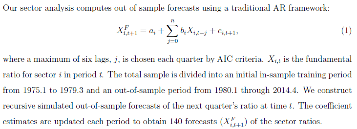
Source: Portfolio Allocations Using Fundamental Ratios: Are Profitability Measures Effective in Selecting Firms and Sectors? Accessed 8/14/17 from SSRN.
So the model forecasts the next quarters multiple, using past multiples (both at the stock and sector level). The portfolios are rebalanced quarterly using the model’s forecasts.
The Results
As mentioned above, the paper examines the model in 3 ways:
- At the sector level (buying the whole sector)
- At the security level (for sector-neutral portfolios)
- At the stock and security level
Following that order (slightly different than the paper), we examine the results below.(2)
Exhibit 2 shows the performance of the model at the sector level. The “average return” below is for each quarter, as the portfolios are rebalanced quarterly. Since there are 10 sectors, the top quintile (20%) is the top 2 sectors, while the bottom quintile is the bottom 2 sectors. As shown below, the forecasts from the model show a spread between the top and the bottom. The long/short portfolio goes long (150% of NAV) the top quintile and shorts (50% of NAV) the bottom quintile. So this L/S portfolio has a net equity position (on a $ basis) of 100% and is somewhat comparable to the SP500 or SP500 EW. Over this same time period, the SP500 returned 3.2% per quarter with a Sharpe ratio of 0.52 and an ending value of $5,455, while the SP500 EW returned 3.3% quarterly with a Sharpe ratio of 0.59% and an ending value of $7,017. Compared to the SP500 and SP500 EW, using the model to forecast sectors has (on average) higher portfolio ending values (before trading costs).
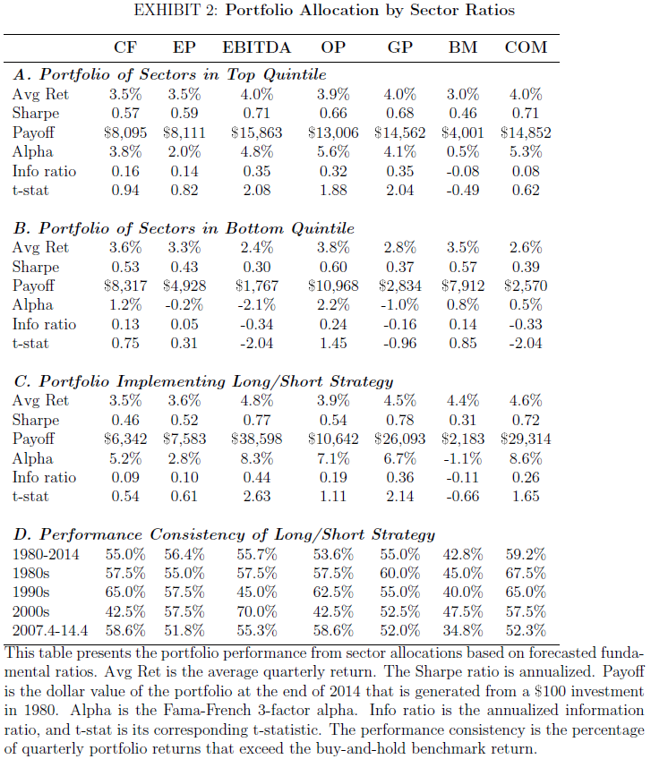
The results are hypothetical results and are NOT an indicator of future results and do NOT represent returns that any investor actually attained. Indexes are unmanaged, do not reflect management or trading fees, and one cannot invest directly in an index. Additional information regarding the construction of these results is available upon request.
Exhibit 3 shows the performance of the model at the firm level while maintaining an equal sector weighting. Again, the paper examines the top and bottom quintiles, while forming a 150/50 L/S portfolio. Compared to the SP500 and SP500 EW, using the model to forecast firm allocations (while holding sectors equal) has higher portfolio ending values (before trading costs). Comparing the model using either (1) sectors or (2) firms, one notices that the model generates more benefit at the firm level than the sector level.
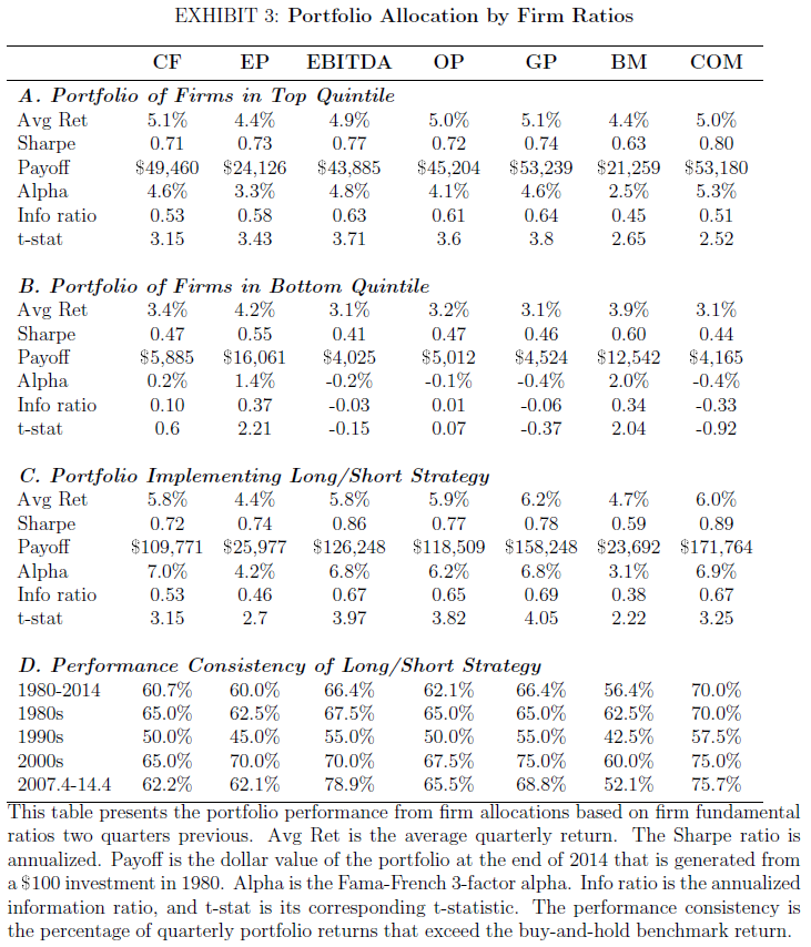
The results are hypothetical results and are NOT an indicator of future results and do NOT represent returns that any investor actually attained. Indexes are unmanaged, do not reflect management or trading fees, and one cannot invest directly in an index. Additional information regarding the construction of these results is available upon request.
Last, what happens if we allow the model to pick both the top sectors and the top firms? Exhibit 1 examines the results to portfolios using either the top (bottom) quintile of sectors (2 sectors), and within the top (bottom) sectors, selects the top (bottom) quintile of firms on the valuation measure. The paper similarly forms the 150/50 L/S portfolios, with a slight difference from the L/S portfolios described above (from footnote 5 in the paper):
(3)A 150/50 strategy takes short positions worth 50% of the portfolio value and uses the proceeds from the shorts to fund long positions worth 150% of the portfolio value. As GICS has ten sectors, short positions are taken in the two sectors in the bottom quintile of valuation so the sectors each have weights of -25%. These funds overweight the sectors in the top quintile of valuation, and these two sectors have weights of 37.5%. The remaining six sectors are equally weighted with each comprising 12.5% of the portfolio.
As such, this long/short portfolio actually allows for allocations to all sectors, while over-weighting the top and under-weighting the bottom, and picks the top (and bottom) firms within each sector. Compared to the SP500 and SP500 EW, using the model to forecast firm allocations (while holding sectors equal) has higher portfolio ending values (before trading costs). Comparing the model using either (1) sectors or (2) firms or (3) sectors and firms, one notices that the model generates the most benefit by being used at both the sector and firm level. The one exception is the book-to-market (B/M) ratio — this measure adds little benefit to the forecast over this time period. In fact, the bottom quintile on B/M for both sectors and firms (the most expensive stocks of the most expensive sectors) outperforms the top quintile on B/M (the cheapest firms from the cheapest sectors) over this time period!
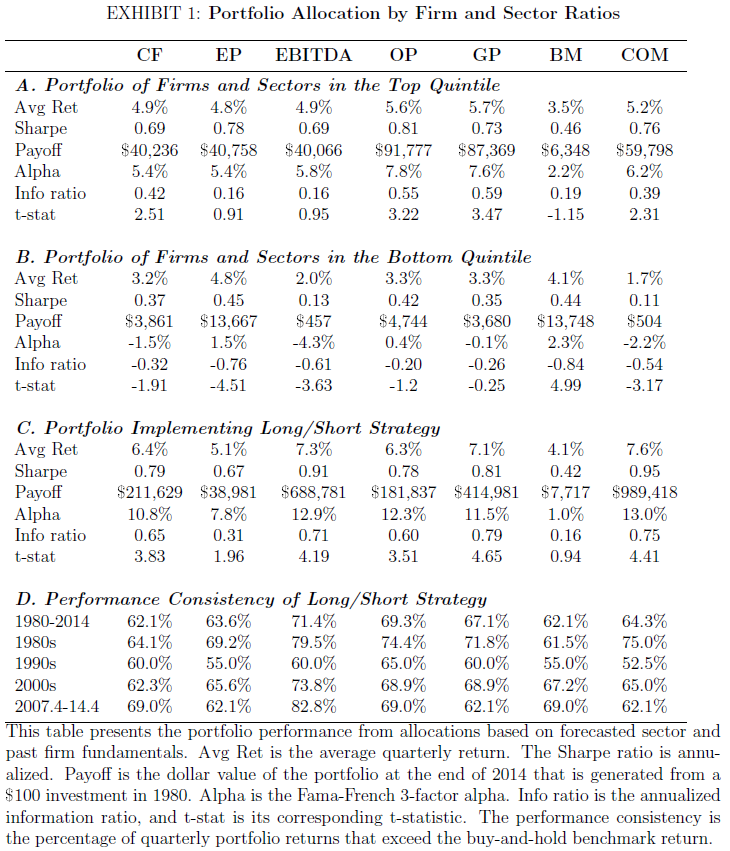
The results are hypothetical results and are NOT an indicator of future results and do NOT represent returns that any investor actually attained. Indexes are unmanaged, do not reflect management or trading fees, and one cannot invest directly in an index. Additional information regarding the construction of these results is available upon request.
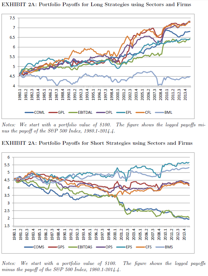
Below the paper shows the payoffs to the long and short portfolios with $0 exposure to the market, by going either long (short) the top (bottom) quintiles on sectors and firms (Exhibit 1), and going short (long) the SP500 Index. As shown below, all portfolios (except book-to-market) have an upward (downward) trend over this time period.
Conclusion
Overall, this paper helps to answer the question of what is the best way to use valuation measures — within sectors, within firms, or both? After examining the data, using the model’s forecasts on multiples works the best at both the firm and sector level, while working the worst at the sector level. The paper also highlights a weird effect within the B/M measure, which adds little value over this time period (albeit these are forecasted B/M multiples, not actual B/M multiples). At the outset, I mentioned that we generally recommend simply buying the cheapest stocks, regardless of the sector. One should note that in this paper, the largest returns are found in the L/S portfolio by over-weighting the cheapest stocks within the cheapest sectors and under-weighting the most expensive stocks within the most expensive sectors — giving credence to our belief to always buy the cheapest stocks, regardless of sector.(4)
Let us know what you think!
Portfolio Allocations Using Fundamental Ratios: Are Profitability Measures Effective in Selecting Firms and Sectors?
- J. Christopher Hughen and Jack Strauss
- A version of the paper can be found here.
Abstract:
Our study assesses the performance of portfolios formed using out-of-sample sector forecasts and past firm fundamental ratios in real time from 1980.1-2014.4. Portfolio allocations based on profitability measures — gross profit, operating profit, and EBITDA — generate performance substantially better than a buy-and-hold benchmark. Long/short portfolio allocations using these fundamentals possess alphas over 14% and increase Sharpe ratios by over 60%. These portfolio strategies consistently beat a buy-and-hold benchmark two-thirds of the time over thirty-five years and over each of the last three decades. A composite variable of profitability measures provides the highest payoff for firm allocations, while strategies using EBITDA are the most profitable for out-of-sample sector allocations. Our results demonstrate that profitability metrics, which use a measure of earnings above net income, are superior indicators of sustainable economic performance, since they are more strongly linked to both future returns and cash flows than net income.
References[+]
| ↑1 | Examining our Quantitative Value and Quantitative Momentum processes, we find that imposing sector constraints lower the CAGR, while reducing tracking error |
|---|---|
| ↑2 | The paper examines the results in the following order: 3, 1, 2 |
| ↑3 | Note it is unclear how the other 150/50 portfolios are formed in the paper. Here is the text on the Sector ratios:
Similarly, here is the text for the firm L/S portfolios:
As such, I assume the previous tables go long (150%) the top portfolio and short (50%) the bottom portfolio |
| ↑4 | Or the stocks with the highest momentum |
About the Author: Jack Vogel, PhD
—
Important Disclosures
For informational and educational purposes only and should not be construed as specific investment, accounting, legal, or tax advice. Certain information is deemed to be reliable, but its accuracy and completeness cannot be guaranteed. Third party information may become outdated or otherwise superseded without notice. Neither the Securities and Exchange Commission (SEC) nor any other federal or state agency has approved, determined the accuracy, or confirmed the adequacy of this article.
The views and opinions expressed herein are those of the author and do not necessarily reflect the views of Alpha Architect, its affiliates or its employees. Our full disclosures are available here. Definitions of common statistics used in our analysis are available here (towards the bottom).
Join thousands of other readers and subscribe to our blog.