- Matúš Padyšák
- Quantpedia.com
- A version of this paper can be found here
- Want to read our summaries of academic finance papers? Check out our Academic Research Insight category
Abstract
While there may be debates about passive and active investing, and even blogs about the numbers of active funds that were outperformed by the market, history taught us that the outperformance of active or passive investing is cyclical. As a proxy for active investing, the paper examines factor strategies and their smart allocation using fast or slow time-series momentum signals, the relative weights based on the strength of the signals, and even blending the signals. While the performance can be significantly improved, factors can still lose to the generic market in both the US and EAFE samples. However, the passive approach did not show to be superior. The factor strategies and market are significantly negatively correlated and impressively complement each other. The combined Smart Factors and market portfolio outperforms both factors and market throughout the sample in both markets.
Introduction
In the equity market, there are two general types of investors: active and passive.(1)
A passive investor simply tracks the market with the lowest tracking error and cost. Thanks to index funds and ETF’s this process is now easy to implement and cheap!
On the other hand, there are active investors, whose aim is to achieve better returns or risk-adjusted returns against a passive benchmark.
Wise passive investors aim for a long horizon and do not panic when they experience their first significant drawdown. But good luck finding these “humans!” That first large drawdown quickly turns all but the most hardcore of passive investors into active investors. It is this tendency that creates a major incentive for active investment management to supply the market with more dynamic investment options.
For our discussion, there is an important subgroup of active investors we must dig into, factor investors. Factor investors seek to gain exposure to specific equity factors including value, size, volatility, momentum, or quality. With numerous ETFs, it is also easy to get exposure to these factors, though it’s important to be sure one is getting the desired exposure (A.K.A. Active Share) and not being a closet passive investor with inadequate exposure to factors.
Note: the author is a non-native English speaker, but a quant investing and education enthusiast…judge accordingly :-)
Finance Nerds Debate
Having established that there are two major management styles and many factors, numerous questions arise.
Firstly, is active or passive investing better?
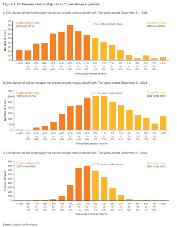
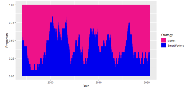
Though both sides love to claim victory and each boastfully stand on their returns, when they are good, the truth is that the outperformance of active and passive investment styles seems to be cyclical, with periods of active (passive) outperformance rotating (see the following figure below). With this, the answer to the question of which investing is better, changes depending on when the question is asked. Ideally, we would find a solution to a different problem, in which state of the market is it better to invest passively, and in which state of the market is it better to invest actively? Once we’ve addressed that we’ll seek to answer whether our rotating between passive and active investing strategy can beat the market on a more consistent basis.
The second question that arises in the halls of finance departments is whether Factor investing is better than “pure” active investing. It is widely recognized that equity factors have cyclical performance. Nearly every factor has gone through a long enough dry spell to be considered “dead.” The argument du jour is that value has been collected by the Grim Reaper of the market efficiency Which has already happened in the past so the value factor may be cat-like with 9 lives, providing some credibility to the cat-like thesis Blitz and Hanauer (2020) claim that value can be resurrected. Momentum is notoriously known for its crashes (Hanauer and Windmüller, 2020). Also, the size factor seems to have its problems (Blitz and Hanauer, 2020). On the other hand, quality appears to be emerging as a popular investment style, and it has even enjoyed outperformance compared to the other factor during the recent first Covid wave (Quantpedia, 2020).
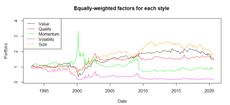
Now that we’ve established that factor investing is not that straightforward and each factor has its own cycle of performance, we hope to use these cycles and find a profitable way to invest across equity factors. The factors in our research have been obtained from the Alpha Architect’s Factor Investing Data Library. We utilize 20 different factors(2) that cover all the major styles: Value, Momentum, Volatility, Quality, and Size. Our paper is going to focus on two markets: the US market that is represented by the top 1500 stocks and the developed market (EAFE).
Since the performance of the factors is cyclical, the hypothesis of the paper is that each factor could be a vital part of the final portfolio. However, the weight of each factor in the portfolio should be changing in time. A possible way to implement this is to react to the actual market situation. Garg et al. (2019) examined time-series momentum strategies and momentum turning points. According to the research, turning points are the Achilles’ heel of time-series momentum portfolios. The reason is straightforward, slow signals tend to be unreactive to changes in trend, and fast signals are often false alarms that lead to the proverbial “Whipsaw.” The authors examine fast and slow momentum signals and different blending approaches to construct more profitable momentum strategies. The weight of the long (short) position depends on both fast and slow signals, and whether they agree or disagree. We follow a similar approach for the construction of the factor momentum strategies, but there are major differences. For the active factor strategy, we first examine two signals: fast, which is 1-month momentum, and slow, which is 12-month momentum. Moreover, we examine a strategy that is traded only if both signals agree and a blended strategy similar to Garg et al. (2019).
We utilize the fast and slow signal separately for each factor, then cross-sectionally rank the absolute value of the signal to obtain the strength of the signal. This ranking system acts like a weighting – the stronger the signal; the greater the weight. After establishing cross-sectional strength, the factor strategies that utilize the slow and fast signals can be further enhanced. The detailed strategies and results can be found in sections 3, 4, and 5.
Our dynamic weighting of factors outperforms the baseline strategies. The outperformance of dynamical weighting compared to all other strategies is present on each market and each type of portfolio sort (quintiles, deciles, and ventiles). Moreover, the results of the dynamic weighting of signals outperform other strategies in two distinct approaches. Firstly, when we consider the relative strength of the signals for all factors together or in the other case when we initially break all the factors into individual investment styles separately. The results are almost exactly the same(3).
It is worth mentioning that by utilizing our strategy the investing process becomes “immune” to problems like value versus growth or short-term momentum/short-term reversals. For example, if value tends to be profitable, the strategy would tilt its exposition to the value factors. If the value tends to be unprofitable (growth is profitable), the strategy shorts the value factors (in other words, it reverses deciles, quintiles, or any other sorted portfolios). Having established that it is possible to utilize the factors better in a relative-strength dynamically weighted factor momentum strategy, it is time to get back to the active versus passive investing debate.
In the recent period, it is well-known that many factors have underperformed.
The first impression would indicate that, in the past, proponents of passive investing were right. However, that conclusion would not be entirely correct. Later, we show that active investing, using the relative-strength dynamically blended factor momentum strategy could be a great addition to the market portfolio. The combined strategy looks back on the past twelve months, and twelve moving averages (MA) of returns: one month, two months, three months, and so on. Suppose the MA for active investing (factor momentum) is larger than MA for market portfolio, then the active investing scores one point. Otherwise, the market portfolio gets one point. Therefore, each month, the weight of the factor momentum and market portfolio is determined by the number of “winning” (losing) moving averages. Combining active and passive investing largely outperforms passive investing only. Moreover, if we have a rule that we follow for investing into factors and the market, it is definitely an active investing strategy.
Although the relative-strength dynamically blended factor momentum strategy and its combination with the market portfolio might seem to be a tangled complicated methodology, the rules are fairly straightforward and transparent. It is possible to ex-post choose the best lookback periods for fast and slow indicators, or the best blending rule, however, such overfitting is not in the interest of this paper. Strategies should be transparent, and the aim of this paper is to show a set of transparent rules to find answers to our two primary questions. Firstly, which factor to invest in (factor allocation problem), and secondly, to have a rule-based solution to the active versus passive clash. The paper is mainly related to the work of Gupta and Kelly (2018), which examines the time-series factor momentum, and the paper of Arnott et al. (2020), which explores the cross-sectional factor momentum strategy. Naturally, the paper is also related to the research on individual factors (which is covered extensively by Alpha Architect).
Data
Factors are obtained from the Alpha Architect’s Factor Investing Data Library. We track twenty different factors(4) which covers all the major styles: Value, Momentum, Volatility, Quality, and Size. All factors are either value-weighted or equally-weighted. We are interested in two markets: the US market that is represented by the top 1500 stocks and the developed market (EAFE). The data spans from Jan 1, 1993, to August 31, 2020, therefore, it includes many major financial crises, e.g. the dot-com bubble, the financial crisis of 2007–2008, the recent COVID crisis (the first wave, including the recovery), and many other market downturns.
Methodology
For each factor 𝑖, at time 𝑡, we first compute the fast and slow momentum signals as follows:
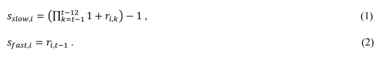
Where 𝑟𝑖,𝑡 denotes the monthly return for month 𝑡 and factor 𝑖, s𝑠𝑙𝑜𝑤,𝑖 is the slow signal, and 𝑠𝑓𝑎𝑠𝑡,𝑖 is the fast signal.
Signals can be used in time-series momentum strategies. We also consider weighted relative-strength signals. The raw weight is found as follows: we take the cross-sectional rank of the signal divided by the sum of all ranks, multiplied by the sign of the signal. The computation can be denoted by the following equation:
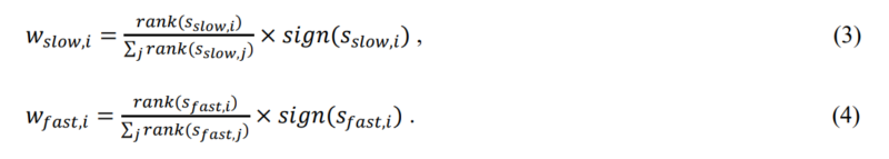
Therefore, the long or short position is scaled by the cross-sectional strength of the signal. The idea is that the stronger signal should have a bigger weight in the portfolio. Moreover, by construction, traditional factor portfolios (long-short) can be flipped. For example, investing in the value factor does not need to consist of a long position in value stocks and a short position in growth stocks, given the equations (1) and (2), the positions can be flipped.
With established signals and weights, we can now form all the variants of examined strategies. Given the equations (1)-(4) there are two options. First, strategies can utilize the signs as signals and factors are equally-weighted in the portfolio. Second, the strategy also employs the raw weights of (3) and (4) to ensure that the factor strategy with a stronger signal gets a larger weight in the portfolio. Throughout the paper, 𝑛 is the number of traded factors.
We next define strategies based on the slow signals and on the fast signals:
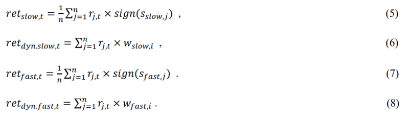
The returns for the neutral strategy or a strategy that only opens positions if both signals agree can be defined as:

The next strategy is a dynamic neutral strategy. The strategy is similar to the blended strategy (8), but it also employs the raw weights of (3) and (4) to ensure that the factor strategy with a stronger signal gets a larger weight in the portfolio.

The blended strategy reduces the weight in the times when the slow and fast indicator do not agree – in the correction state (when the slow signal is positive but the fast is negative) or in the rebound state (when the slow signal is still negative, but the fast is already positive). In the correction state, there is not a “full” short position, but the weight is scaled to half (the weight of the factor is -0.5). In the rebound state, there is not a “full” long position, but the weight is scaled to half again (the weight of the factor is 0.5).

The final strategy is the dynamically blended strategy.

Combined Strategy
In the introduction, we outlined that passive market investing has outperformed factor investing. In this section, we show that it might be even better to combine the previously mentioned dynamically blended factor momentum strategy and the market portfolio. The combination is straightforward, the combined strategy looks back on the past twelve months, and twelve-month MA’s of the returns. If the MA for active investing (factor momentum) is larger than the MA for the market portfolio the active investing scores one point. Otherwise, the market portfolio gets one point. Therefore, each month, the weight of the factor momentum and market portfolio is determined by the number of “winning” (losing) moving averages. At time t, the weight of the market portfolio and factor portfolio (fport) is given by the following equations:
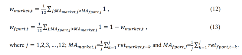
Return of the combined portfolio at month 𝑡 is equal to:

Results
Throughout the research, results were qualitatively the same for both weight options: The equally-weighted or value-weighted stocks in each of the factors did not change the results. Therefore, only the value-weighted individual factors are examined in the proposed strategies. Also, the sorting method (deciles, quintiles, ventiles) did not largely change the results, and the results were qualitatively the same. While the individual needs for diversification can significantly influence the number of traded stocks, the study opts for deciles as a “middle ground”. The results are divided into two sections: for US stocks and for international EAFE stocks.
Results – US stocks
| Strategy | Return | Volatility | Max Drawdown | Risk-adjusted performance |
| Slow | 3.362% | 10.969% | -38.075% | 0.306 |
| Fast | 3.235% | 11.032% | -24.445% | 0.293 |
| Neutral | 3.547% | 8.464% | -22.83806% | 0.419 |
| Dynamically neutral | 4.402% | 11.224% | -27.783% | 0.392 |
| Blended | 3.451% | 9.183% | -20.911% | 0.376 |
| Dynamically blended | 4.235% | 12.133% | -26.303% | 0.349 |
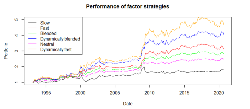
Table 1 Performance metrics for strategies mentioned in section 3 in the US market. Returns and volatilities are annualized. Risk-adjusted performance is return divided by volatility. The sample consists of returns for the period of 31.12.1992 to 31.8.2020. Individually, each factor is value-weighted. The factor portfolios are weighted according to section 3. The Slow is the long term momentum signal (12 months), Fast signal is the short term momentum signal (1 month), Neutral trades only if both signals agree, Blended strategy reduces the weight in the times when the slow and fast indicator do not agree (equation 11). Dynamic strategies employ relative weights (the strength of each signal – equations 3 and 4)
The results are hypothetical results and are NOT an indicator of future results and do NOT represent returns that any investor actually attained. Indexes are unmanaged, do not reflect management or trading fees, and one cannot invest directly in an index.
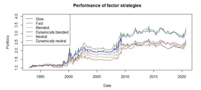
The dynamical approach improves the performance of both neutral and blended strategies. However, by the construction, both strategies are blended with different weights for short and fast signals. As expected, dynamic strategies are the most profitable. The blending of the signals adds some performance (measured by the returns) compared to slow or fast signals. Therefore, the blending of time-series factor momentum signals seems to be profitable. Even larger returns were obtained with dynamic strategies that are similar to the cross-sectional momentum.
The performance can also be inspected visually, by looking at the equity lines for the unit portfolios.
The results are hypothetical results and are NOT an indicator of future results and do NOT represent returns that any investor actually attained. Indexes are unmanaged, do not reflect management or trading fees, and one cannot invest directly in an index.
All of the strategies are profitable, do not have large drawdowns or volatilities, but they do not seem to be that profitable. There are many periods where the performance is flat.
The results are hypothetical results and are NOT an indicator of future results and do NOT represent returns that any investor actually attained. Indexes are unmanaged, do not reflect management or trading fees, and one cannot invest directly in an index.
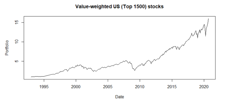
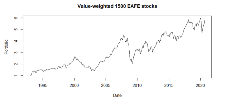
Compared to long/short factor strategies, a buy-and-hold beta approach for the top 1500 US stocks would have skyrocketed.
A natural question arises, is there any reason to invest in factors?
Common knowledge is that the outperformance of active and passive investing is cyclical. The edge changes based on market conditions. Therefore, we suggest that both the active factor strategy and market portfolio should be utilized in the investor’s portfolio. However, there needs to be set a rule for the allocations. The Spearman’s correlation coefficient between the market portfolio and dynamically blended strategy is -0.185 (p-val 0.0006969). The coefficient between dynamically neutral strategy and market portfolio is -0.143 (p-val 0.009194). Both correlations are negative and highly statistically significant using non-parametric (therefore robust in this case) tests. These results suggest that it should be beneficial to combine those strategies. The performance of active and passive investing is cyclical and slightly negatively correlated. The straightforward rules based on simple moving averages were established in section 4.
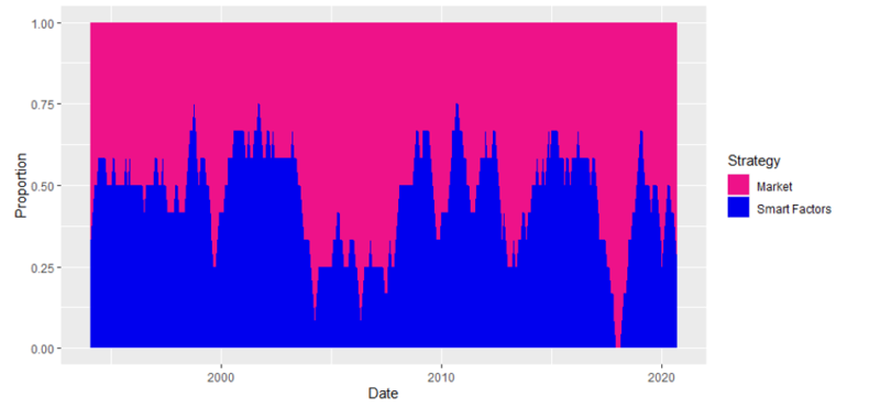
Throughout the next section, the combination is presented for the market portfolio and dynamically blended strategy, which we call “Smart Factors.”
and market portfolio (Market) using a combined approach from section 4. US market
The results are hypothetical results and are NOT an indicator of future results and do NOT represent returns that any investor actually attained. Indexes are unmanaged, do not reflect management or trading fees, and one cannot invest directly in an index.
| Strategy | Return | Volatility | Max Drawdown | Risk-adjusted performance |
| Smart Factors | 3.884% | 12.282% | -26.303% | 0.316 |
| Market | 10.519% | 15.086% | -50.007% | 0.697 |
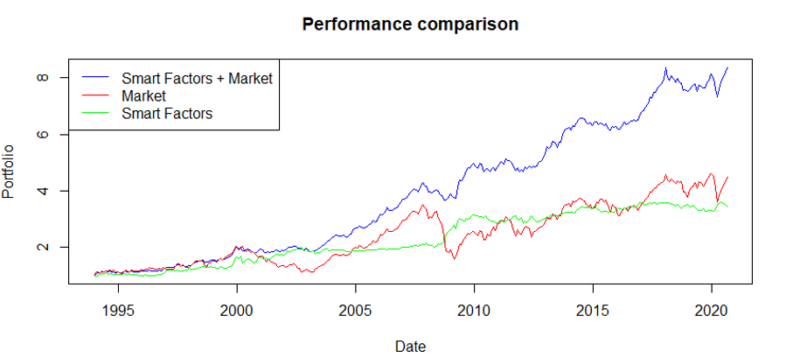
| Smart Factors + Market | 11.909% | 10.460% | -16.95% | 1.138 |
Table 2 Performance metrics for strategies mentioned above in the US market. Returns and volatilities are annualized. Risk-adjusted performance is return divided by the volatility. The sample consists of returns for the period of 31.12.1993 to 31.8.2020.
The results are hypothetical results and are NOT an indicator of future results and do NOT represent returns that any investor actually attained. Indexes are unmanaged, do not reflect management or trading fees, and one cannot invest directly in an index.
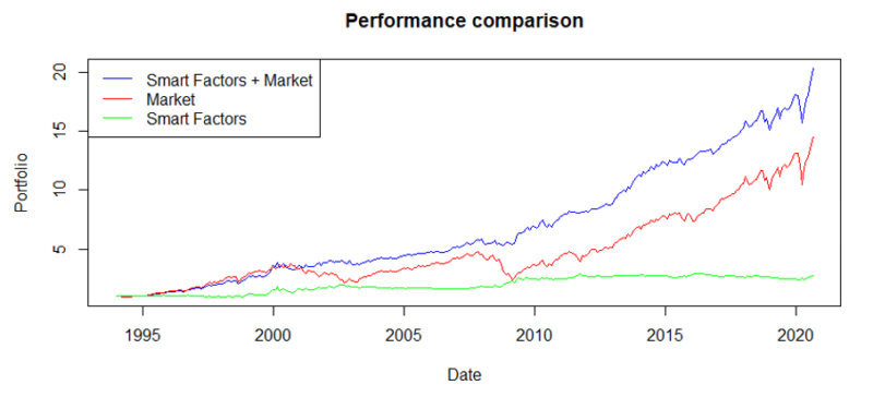
The combination of Smart Factors + market demonstrates the potential of factor strategies. Gathering information from Figure 1-3, factors are profitable when the market is not, and by construction (section 4), the combination strategy has the biggest allocation into factors when there is a market downturn. On the other hand, the factors tend to be flat when the market is largely profitable. As a result, the combination has the largest return, the lowest volatility and max drawdown, and the highest risk-adjusted performance. A dollar invested in the 12.31.1993 would result in 20.28 dollars by the 8.31.2020 compared to only 14.52 dollars for the Market portfolio.
The results are hypothetical results and are NOT an indicator of future results and do NOT represent returns that any investor actually attained. Indexes are unmanaged, do not reflect management or trading fees, and one cannot invest directly in an index.
The results are hypothetical results and are NOT an indicator of future results and do NOT represent returns that any investor actually attained. Indexes are unmanaged, do not reflect management or trading fees, and one cannot invest directly in an index.
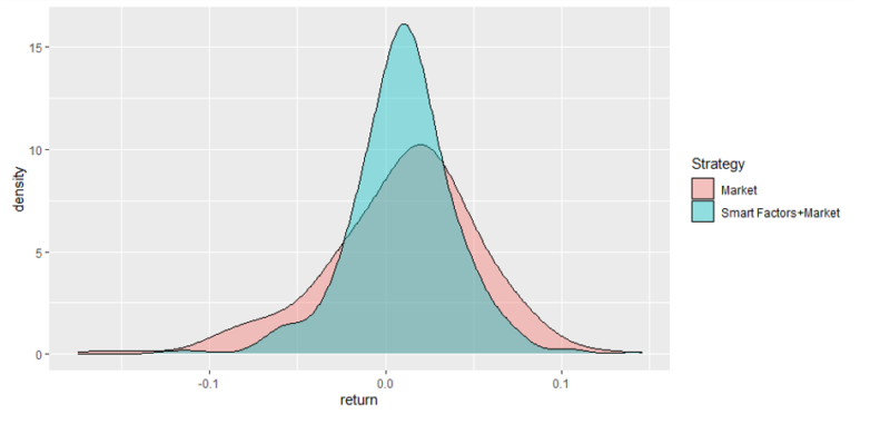
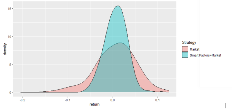
Returns of the combination strategy also tend to be more favorably distributed. The left tail is shorter and thin, not as heavy as for the market portfolio. As expected, the same can be said about the right tail, but overall, the combination is better.
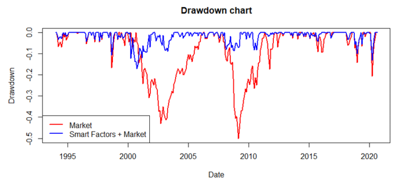
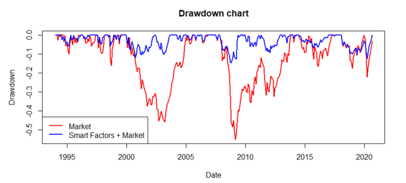
The list of favorable properties does not end; the following chart shows the much lower drawdowns for the combined portfolio. While one could say that the passive approach is better than some factor (smart beta) strategies, and passive investing is superior to the active, their active combination and dynamic allocation largely outperform the passive buy-and-hold approach of the market.
The results are hypothetical results and are NOT an indicator of future results and do NOT represent returns that any investor actually attained. Indexes are unmanaged, do not reflect management or trading fees, and one cannot invest directly in an index.
Results – EAFE stocks
| Strategy | Return | Volatility | Max Drawdown | Risk-adjusted performance |
| Slow | 2.182% | 7.195% | -28.947% | 0.303 |
| Fast | 4.188% | 8.021% | -13.069% | 0.522 |
| Dynamically fast | 5.701% | 10.813% | -15.369% | 0.527 |
| Neutral | 3.301% | 5.874% | -17.062% | 0.562 |
| Blended | 3.773% | 6.598% | -11.082% | 0.572 |
| Dynamically blended | 5.165% | 8.917% | -14.599% | 0.579 |
Table 3 Performance metrics for strategies mentioned in section 3 in the EAFE stocks. Returns and volatilities are annualized. Risk-adjusted performance is return divided by volatility. The sample consists of returns for the period of 31.12.1992 to 31.8.2020. Individually, each factor is value-weighted. The factor portfolios are weighted according to section 3. The Slow is the long term momentum signal (12 months), Fast signal is the short term momentum signal (1 month), Neutral trades only if both signals agree, Blended strategy reduces the weight in the times when the slow and fast indicator do not agree (equation 11). Dynamic strategies employ relative weights (the strength of each signal – equations 3 and 4).
The results are hypothetical results and are NOT an indicator of future results and do NOT represent returns that any investor actually attained. Indexes are unmanaged, do not reflect management or trading fees, and one cannot invest directly in an index.
The performance of strategies in the EAFE universe is comparable to the US sample. However, the fast signals tend to be significantly more profitable, indicating that the short-term factor momentum outperforms the long-term factor momentum. On a risk-adjusted basis, the dynamically blended strategy is the winner.
The results are hypothetical results and are NOT an indicator of future results and do NOT represent returns that any investor actually attained. Indexes are unmanaged, do not reflect management or trading fees, and one cannot invest directly in an index.
The results are hypothetical results and are NOT an indicator of future results and do NOT represent returns that any investor actually attained. Indexes are unmanaged, do not reflect management or trading fees, and one cannot invest directly in an index.
The case is not the same as in the US market, the EAFE market portfolio has not skyrocketed compared to the long/short factor strategies. The market portfolio is very volatile compared to the factors, and the returns are similar. Spearman’s correlation coefficient between the market portfolio and dynamically blended strategy is -0.122 (p-val 0.02661). Therefore, the result is the same as in the US case. The correlation is slightly negative and statistically significant. These results point to the same conclusion as in the US case. It should be beneficial to combine those strategies. The straightforward rules based on simple moving averages were established in section 4.
Throughout the next section, the combination is presented for the market portfolio and dynamically blended strategy that would be called “Smart Factors.”
and market portfolio (Market) using a combined approach from section 4. EAFE market
The results are hypothetical results and are NOT an indicator of future results and do NOT represent returns that any investor actually attained. Indexes are unmanaged, do not reflect management or trading fees, and one cannot invest directly in an index.
| Strategy | Return | Volatility | Max Drawdown | Risk-adjusted performance |
| Smart Factors | 4.708% | 8.944% | -14.599% | 0.473 |
| Market | 5.769% | 15.957% | -55.15% | 0.361 |
| Smart Factors + Market | 8.264% | 8.308% | -14.747% | 0.995 |
Table 4 Performance metrics for strategies mentioned above in the EAFE market. Returns and volatilities are annualized. Risk-adjusted performance is return divided by the volatility. The sample consists of returns for the period of 12.31.1993 to 8.31.2020.
The results are hypothetical results and are NOT an indicator of future results and do NOT represent returns that any investor actually attained. Indexes are unmanaged, do not reflect management or trading fees, and one cannot invest directly in an index.
Results are similar to the US market; factors are largely profitable when the market is in the downturn. A great example of this is the time period after the year 2000, the factor strategies had one of the best periods, while the market is suffered. A similar situation is found before 2010. Therefore, the factors and markets complement each other and using straightforward rules, and the active approach beats the market again.
The results are hypothetical results and are NOT an indicator of future results and do NOT represent returns that any investor actually attained. Indexes are unmanaged, do not reflect management or trading fees, and one cannot invest directly in an index.
The density plot and drawdown chart bear the same results as in the US case. The density plot even shows that the left tail is even heavier than in the US case. However, the tail disappears when the strategies are combined. Moreover, the distribution of monthly returns of Smart Factors + Market evokes the normal distribution, and we cannot reject the null hypothesis (Shapiro–Wilk test) that returns are normally distributed on the 1% significance level. The mean monthly return is 0.69%.
The results are hypothetical results and are NOT an indicator of future results and do NOT represent returns that any investor actually attained. Indexes are unmanaged, do not reflect management or trading fees, and one cannot invest directly in an index.
The results are hypothetical results and are NOT an indicator of future results and do NOT represent returns that any investor actually attained. Indexes are unmanaged, do not reflect management or trading fees, and one cannot invest directly in an index.
Conclusion
We conclude that the results are qualitatively the same for both investment universes. In both EAFE and US stocks, the market portfolio (which includes beta) outperforms long/short factor strategies. The results hold even if we use time-series, cross-sectional factor momentum, or blending the fast and slow momentum signals. However, the blending of the fast and slow signals proved to be superior to using the fast or slow signals only. Overall, the results are in line with the known results for momentum anomalies in the individual stocks.
It might look like the passive approach of buy-and-hold market indices outperforms active investing, and that active investing is pointless, but we show that active investing can hold promise. The active approach that consists of smart allocation into both Smart Factors strategy and market portfolio significantly outperforms either market or factors. Smart Factors and market are in both cases, slightly negatively correlated. The performance of both is cyclical, and factors have generated performance during market downturns. Therefore, by allocating into market and factors using a scoring system based on moving averages, it is possible to create a much more profitable portfolio, with lower volatility or drawdowns.
These results are applicable to both markets – US and EAFE. In both cases, the risk-adjusted return dramatically improves switching from market portfolio to the combined portfolio (from 0.361 to 0.995 for EAFE stocks and from 0.697 to 1.138 for US stocks). Lastly, comparing the factors and markets, the EAFE factors outperform US factors, but US market outperforms the EAFE market. Therefore, the combined portfolio in the connected samples could be an interesting idea for further research.
Related literature
[1] Arnott, Robert D. and Clements, Mark and Kalesnik, Vitali and Linnainmaa, Juhani T., Factor Momentum (February 1, 2019). [2] Blitz, David and Hanauer, Matthias Xaver, Resurrecting the Value Premium (October 15, 2020). [3] Blitz, David and Hanauer, Matthias Xaver, Settling the Size Matter (September 4, 2020). [4] Christopher B. Philips, CFA; Francis M. Kinniry Jr., CFA; David J. Walker, CFA: The Active-Passive Debate: Market Cyclicality and Leadership Volatility (July 2014). Vanguard research. [5] Garg, Ashish and Goulding, Christian L. and Harvey, Campbell R. and Mazzoleni, Michele, Momentum Turning Points (December 9, 2019). [6] Gupta, Tarun and Kelly, Bryan T., Factor Momentum Everywhere (November 1, 2018). Yale ICF Working Paper No. 2018-23 [7] Hanauer, Matthias Xaver and Windmüller, Steffen, Enhanced Momentum Strategies (August 07, 2020). [8] Quantpedia: YTD Performance of Equity Factors – Update After Two Months (15.May 2020). Quantpedia’s blog.
References[+]
| ↑1 | terms are described here. |
|---|---|
| ↑2 | The factors include: Asset Growth, Beta, Book/Price, Cash Flow/Price, Debt Paydown Yield, Dividend/Price, Earnings/Price, EBIT/TEV, EBITDA/TEV, Financial Strength Score, Gross Profit, various Momentum measures (1m, 6m, 12m and 12m with the last month skipped), Repurchase Yield, Return on Assets, Return on Equity, Sales/Price, Shareholder Yield, Shareholder Yield with Debt, Size and Volatility. |
| ↑3 | since breaking the factors into individual styles does not alter the results, for simplicity, results for such variants are unpublished |
| ↑4 | Asset Growth, Beta, Book/Price, Cash Flow/Price, Debt Paydown Yield, Dividend/Price, Earnings/Price, EBIT/TEV, EBITDA/TEV, Financial Strength Score, Gross Profit, various Momentum measures (1m, 6m, 12m and 12m with the last month skipped), Repurchase Yield, Return on Assets, Return on Equity, Sales/Price, Shareholder Yield, Shareholder Yield with Debt, Size and Volatility |
About the Author: Matus Padysak
—
Important Disclosures
For informational and educational purposes only and should not be construed as specific investment, accounting, legal, or tax advice. Certain information is deemed to be reliable, but its accuracy and completeness cannot be guaranteed. Third party information may become outdated or otherwise superseded without notice. Neither the Securities and Exchange Commission (SEC) nor any other federal or state agency has approved, determined the accuracy, or confirmed the adequacy of this article.
The views and opinions expressed herein are those of the author and do not necessarily reflect the views of Alpha Architect, its affiliates or its employees. Our full disclosures are available here. Definitions of common statistics used in our analysis are available here (towards the bottom).
Join thousands of other readers and subscribe to our blog.