We are proponents of focused (i.e., 50 stock) long-only value and momentum factor strategies.(1) There are also plenty of incredibly talented systematic investing shops that build highly diversified factor portfolios with 500+ stocks. We take no stance on the “best” approach to portfolio construction because there is no “best” approach: the reality is that each approach has costs and benefits.
Our belief is that concentrated value and momentum factor portfolios(2) can deliver higher expected returns relative to diluted factor portfolios because these portfolios are more concentrated in the characteristic that drives risk/return (ie. low p/e stocks or recent winners). And because these concentrated constructs deliver more factor exposure, they also deliver more factor risk. So if an investor has a 10yr+ investment objective and a capacity to bear the risk (and tracking error!), we believe our strategies are a good fit, but they are not for everyone. In short, we do not believe in free lunches.
Nonetheless, every so often a reader will show us the research paper, “How Diversification Impacts the Reliability of Outcomes.” Readers who glance through this paper, without understanding the portfolio construction model deployed and/or the underlying inputs, typically walk away with this message: by simply adding more stocks to one’s factor portfolios, one can more “reliably” beat the market. Honestly, it sounds like the holy grail of investing.
But then, let’s think for a moment–if one really believes that a “factor” works (and we know it did historically), why would taking a “smaller” bet on the factor increase the probability of beating the market?(3)
To answer that question, we wrote this article on portfolio construction.
Portfolio construction study: main tenets
In this study, we use the exact same model from the paper mentioned above. The only difference is that we use historical empirical estimates for all the inputs of the model for various factor portfolios. The model suggests that when using historical empirical estimates for all the inputs, simply adding more stocks does not substantially increase the probability of beating the market for Value and Momentum. In addition, in a comparison of factor portfolios with varying Ns, the model suggests that concentrated factor (Value and Momentum) portfolios reliably outperform more diversified factor portfolios.
Here is a formal abstract of our key findings:
We identify the relationships between the number of stocks in a factor portfolio and the long-term probability of beating the market (“reliability”). We use a simple model that assumes investment growth is lognormally distributed. The inputs to this model are the following: mean, standard deviation, and correlations. Using historical estimates for the inputs, the model finds that the reliability of value and momentum portfolios is similar across concentrated and diversified constructs. The model also finds that concentrated value and momentum portfolios reliably outperform their diversified counterparts over longer time horizons. This result stems from the fact that concentrated value and momentum portfolios have higher historical mean returns than more diversified value and momentum portfolios.
A PDF version of this is available here.
How Does Diversification Impact the Reliability of Outcomes?
Wei Dai Ph.D. presents a very interesting paper called, “How Diversification Impacts the Reliability of Outcomes.” This paper’s finding is that diluted factor portfolios can more reliably beat the market relative to concentrated factor portfolios, under the assumption that all portfolios have similar average returns. The portfolio construction model presented is powerful and allows researchers to address numerous questions related to factors.(4)
Below, we expand upon Wei Dai’s research and examine four specific research questions using the model presented in Dr. Dai’s paper:
- We first explore the model used in the paper so readers understand how it works and the assumptions required.
- We use the model to explore the small-cap effect and examine the performance of small-cap stocks (Russell 2000 Index) relative to the “market” (Russell 1000 Index).
- We input historical returns, volatility, and correlations into the model.
- The model suggests that one should NOT expect smaller stocks to beat the market. The probability is around 50/50–pretty much a coin flip.
- Second, with some knowledge of how the model works, we examine how to use the model to determine the “reliability” of a portfolio’s ability to “beat the market.” Importantly–we assume expected returns are the same across all portfolios–since the exposure to the size, value, and profitability premiums are the same for all portfolios. This is in contrast to what we did in the first test, where we inputted historical estimates for returns, volatilities, and correlations.
- Under the ‘equal returns’ assumption, the model suggests that simply adding more and more stocks to a portfolio increases the reliability of outperformance.(5)
- The intuition is simple: holding average returns constant, increasing (1) volatility and (2) tracking error will create more dispersion in outcomes.
- Third, we explore specific factor portfolios that are commonly used: value, momentum, and low beta. However, we DO NOT assume that all portfolios have the same average returns. Instead, we use historical estimates for returns, volatility, and correlations. Using historical estimates is important because estimates of factor portfolio returns are strongly related to construction and the factor itself.
- The model suggests that more diversified (1) Value and (2) Momentum portfolios are NOT able to substantially increase the probability of beating the market (i.e. are not more reliable) compared to more concentrated Value and Momentum portfolios. This result is in direct contrast to the paper’s original findings.
- The results for low beta portfolios are different. More diversified portfolios increase the probability of beating the market, which is similar to the original message in the Dai paper. Why is that the case? Low beta portfolios, regardless of construction, generate similar average returns, so relying on the assumption that returns are equal across portfolio constructs approximates reality.
- Bottom line: statements about reliability are highly contingent on the factor under investigation and expected return assumptions.
- Last, we explore the reliability of concentrated portfolios beating diversified portfolios in the context of value and momentum strategies.
- Here, we invert the question–what is the chance that a 200-stock Value/Momentum portfolio beats a 50-stock Value/Momentum portfolio?
- The model suggests that concentrated factor portfolios more reliably beat diversified factor portfolios.
- We also highlight some additional reasons for concentration in the Value and Momentum factors.
Let’s dig into the details.
Below we dig into the four research questions above in more detail.
Section 1: The Portfolio Reliability Model
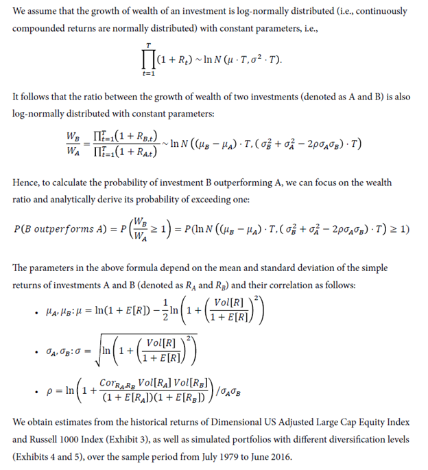
The model used to estimate the probability of outperforming the market in the paper, “How Diversification Impacts the Reliability of Outcomes” by Wei Dai, PhD. is found in the appendix of the paper. We have copied the exact model in this reference below.(6)
No portfolio construction model is perfect, but this model is simple and efficient. With a few parameters (and assuming the growth of wealth is log-normally distributed), we can estimate the probability of one strategy outperforming another strategy over a given course of time (which we can vary).
So what does “reliability” really mean? It is the output
Reliability is defined as the probability that the growth of investment A (i.e., 50 stock value portfolio) is greater than the growth of wealth of investment B (i.e., the “market”) over a given time period.
In other words, “reliability” is the output (probability) of the model.
What are the variables one needs to generate the probability of outperformance?
We need to generate three summary statistics for the model:
- The average monthly return (the arithmetic mean) on the assets under comparison
- The monthly standard deviation of the comparison assets
- The correlation between the comparison assets
So how does the model work?
Well, simply put, we are using the model to compare the ratio of the growth of wealth between two return series.
We need three inputs, and these inputs are very important to the outcome.
Let’s go through each of them and discuss the impact that they have on the results:
- Mean: The model will examine the difference between the means of the two portfolios you are comparing. So if the means are exactly the same, the model should generate a probability near 50% (i.e. a coin toss). If we increase the differences between the two means, holding everything else the same, we increase the probability. If we decrease the differences between the two means, holding everything else the same, we decrease the probability.
- Standard deviation: If we increase the standard deviation, holding everything else the same, we decrease the probability. If we decrease the standard deviation, holding everything else the same, we increase the probability.
- Correlation: If we increase the correlation, holding everything else the same, we increase the probability. If we decrease the standard deviation, holding everything else the same, we decrease the probability.
Simply put, each of the three inputs into the model will affect the probability of outperformance, or the reliability of the outcomes.
To state otherwise is to ignore math.
All of the inputs matter.
Now that we have a baseline understanding of how the model works, let’s take a simple example—What is the probability that small-cap stocks (the Russell 2,000) beat large-cap stocks (the Russell 1,000)?
Below we share the summary statistics using index return data from 1/1/1979 through 2/28/2021:
| Monthly Mean (Arithmetic Avg.) | Monthly Volatility | |
| Russell 1000 (R1K) | 1.06% | 4.41% |
| Russell 2000 (R2K) | 1.10% | 5.70% |
The correlation between R1K and R2K is 0.865804.
So what happens when we put this into the model? What is the probability that small-cap beat large-cap stocks?
We show the results below using the portfolio construction model.
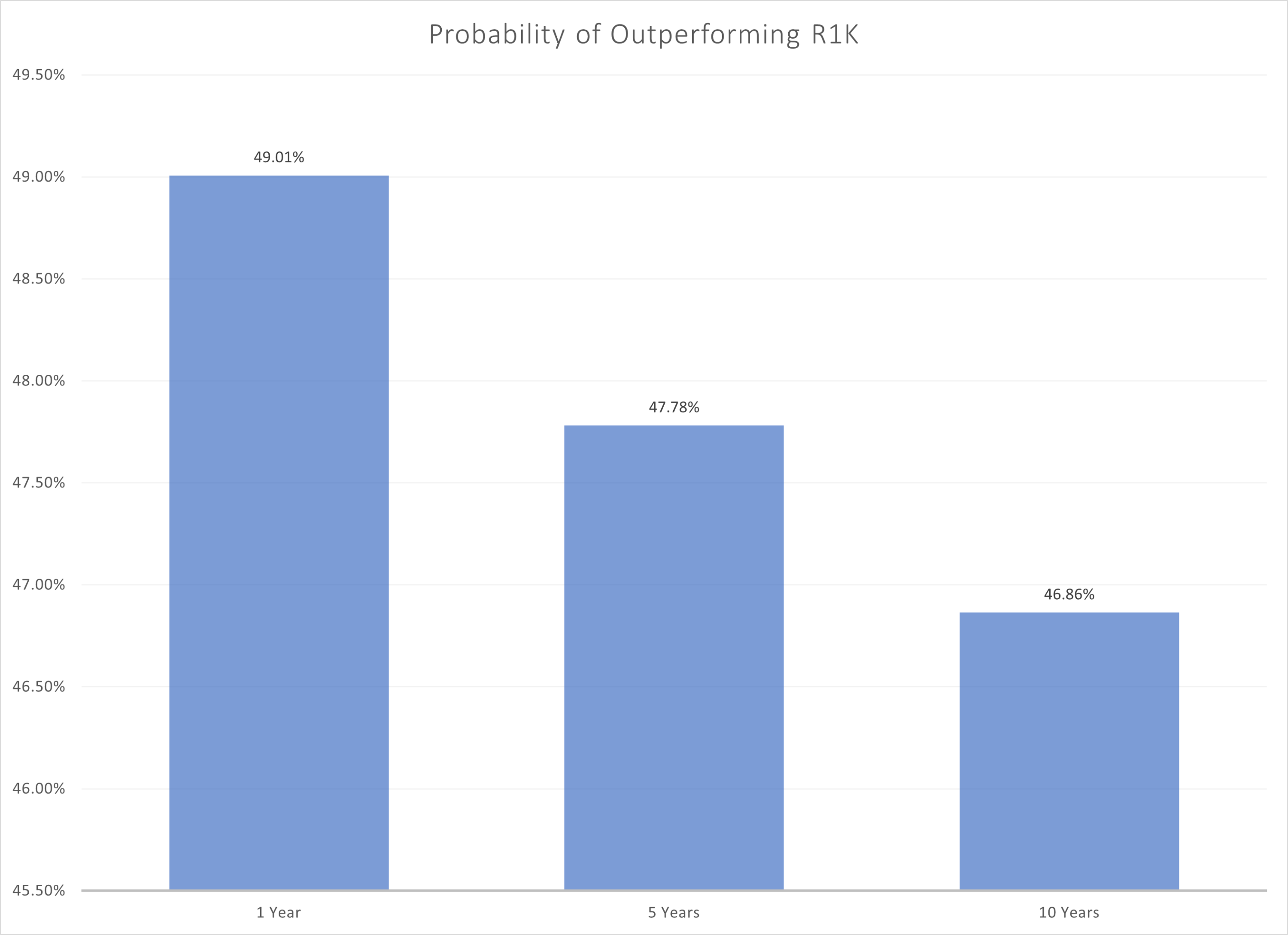
Source: Author’s Calculations. The results are hypothetical results and are NOT an indicator of future results and do NOT represent returns that any investor actually attained. Indexes are unmanaged and do not reflect management or trading fees, and one cannot invest directly in an index.
As we see, the probability at the 1-year, 5-year, and 10-year time horizon is near, but slightly below, 50%. In other words, the model would predict close to a toss-up: small-caps don’t reliably beat large-caps. If anything, there is a small chance of small-caps underperforming large caps over longer horizons.
The result is intuitive given that the historical average monthly returns are very similar, but the volatility is slightly higher for small caps. All else equal, if we have similar returns but more volatility, we would expect a wider dispersion of outcomes for the more volatile asset class (e.g., small-cap stocks) relative to the lower volatility asset (e.g., large-cap stocks). The results above are based on a simple model that uses inputs based on the historical data for the R2K and R1K.
Of course, investors often add a value tilt to their small-cap bet in hopes of improving the average returns.(7) If the model under analysis is well-specified, we would expect that the story might change because tilting towards value stocks within small-caps has historically increased the mean return. We investigate how different mean returns affect the model’s predictions in Section 3.
So now that we have an idea of how the model works, let’s dig into some of the details while varying the number of stocks.
Section 2: What Happens if We Vary the Number of Stocks?
Now we focus on using the model, but we vary the number of stocks in the portfolio. The paper finds that simply adding more stocks increased the ex-ante probability of beating the market–a great outcome, if true!
But how is that result achieved? We replicate the results from the original paper below to answer this question.
From July 1979 through June 2016, the mean (average monthly return) is 1.01% for the market and 1.07% for the Value portfolio (Dimensional US Adjusted Large Cap Equity Index) with a correlation of 0.997–these are the summary statistics from the paper.
From this index, the paper uses simulations while varying the number of stocks, to generate the monthly statistics for portfolios of different sizes.
Exhibit 4 highlights the volatility and tracking error of concentrated and diversified portfolios.
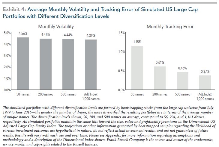
Source Paper: “How Diversification Impacts the Reliability of Outcomes” by Wei Dai, PhD.
As we would expect, portfolios with fewer stocks have the following characteristics:
- A slightly higher monthly volatility
- More tracking error
But what about the expected returns to these different portfolios? Unfortunately, there is not a transparent discussion on this point within the paper. But there are some clues. In the paper, the author highlights that the portfolios are designed to maintain similar exposure to the size, value, and profitability premiums. The mean monthly returns to these portfolios are never specified explicitly in the paper, but it is reasonable to assume that because the characteristics are matched across portfolios, the mean returns will be similar.(8) For replication purposes, we will assume the expected returns are the exact same.
Here are the inputs used in our replication:
- The average return is assumed to be the same for the 50-stock, 200-stock, 500-stock, and 1,000 stock portfolios. We use the Dimensional US Adjusted Large Cap Equity Index mean of 1.07%. For the Russell 1,000 index, we use 1.01%, which is referenced in the paper.
- Exhibit 4 (above) of the paper gives the monthly volatility for each portfolio, which we input into the model.
- We use the following estimated correlations:
- 50-stock portfolio = 0.9670
- 200-stock portfolio = 0.9900
- 500-stock portfolio = 0.9945
- 1000-stock portfolio = 0.9963
It should be noted that the correlations are estimated from index data and are not given in the paper (the paper only gives the tracking error).
We generate the following probabilities of outperformance using the model:
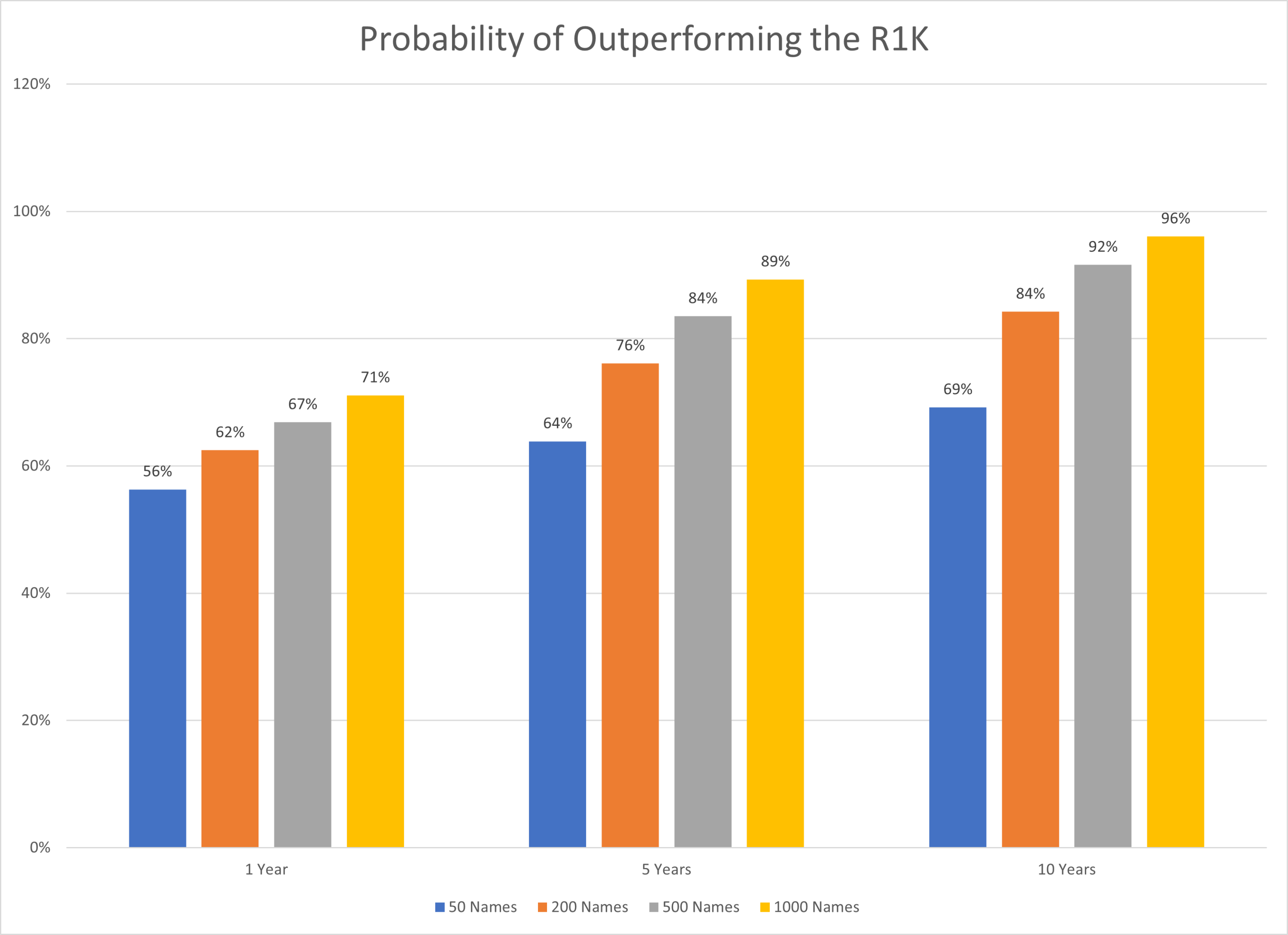
Source: Author’s Calculations. The results are hypothetical results and are NOT an indicator of future results and do NOT represent returns that any investor actually attained. Indexes are unmanaged and do not reflect management or trading fees, and one cannot invest directly in an index.
Our replication results almost perfectly match those presented in the paper.
The takeaway about portfolio construction is exactly the same as is found in the paper: simply adding more stocks to a portfolio increases the probability of beating the market.
But why?
Well, it’s simple math.
Given a lognormal distribution–if we assume the mean is similar across portfolios–but we either (1) increase the volatility or (2) decrease the correlation across portfolios, by design, we lower the probability of outperforming, all else equal.
As we saw above:
- Fewer stocks in the portfolio have higher volatilities. Thus, by definition, they will have a lower probability of beating the market if we keep the mean the same.
- Fewer stocks in the portfolio have a larger tracking error, so they have lower correlations. Thus, by definition, they will have a lower probability of beating the market if we keep the mean the same.
So the results are not surprising once one digs into the model and has a basic understanding of statistics.
However, here is the most important point. All of this analysis hinges on a VERY important assumption–the mean returns across portfolios are held constant.
But what happens if the mean return varies with the number of stocks? For example, should we assume a 50-stock Value portfolio had the same historical mean as a 950-stock Value portfolio?
Of course not.(9)
If one believes that characteristics and/or factors drive expected returns (i.e. you believe Value is a factor), one can’t simultaneously believe that more concentrated factor portfolios have lower expected returns than diluted factor portfolios. Intuitively, a portfolio of the cheapest 50 stocks will mechanically be more exposed to ‘value’ than a portfolio of the cheapest 950 stocks.
We can examine this in granular detail for different portfolios and for different investment factors.
Section 3: What if Portfolio Means Are Allowed to Vary?
We have previously examined the impact that portfolio construction has on Value portfolios and the impact that portfolio construction has on Momentum portfolios. The evidence is pretty clear and the intuition is obvious: historically, more concentrated Value and Momentum portfolios delivered higher expected returns, as well as (1) higher volatility and (2) higher tracking error. Once again highlighting, there are pros and cons to such approaches.
Nonetheless, we ask the question again:
What is the historical performance of value, momentum, and low beta for different portfolio sizes?
Factor 1: Value
To test the Value factor, we generate the universe of the 1,000 largest firms from 7/1/1971 through 12/31/2020. Every month, the 1,000 largest firms are chosen. Financials are excluded for this factor(10) as we are using EBIT/TEV as our Value factor and operating income for a financial company is different than for a non-financial company.(11)
Every month, we simply pick the top N names on Value.
We allow the number of stocks (N) to vary from a 15 stock portfolio up to the top 950 stocks on Value–in other words, the 950-stock portfolio picks all but the 50 most expensive stocks on EBIT/TEV.
We also allow the rebalance frequency to vary. It can range from 1 month to 12 months. For portfolios held over 1 month, overlapping portfolios are formed (referred to as ‘traunching’ by practitioners).
The portfolios are then either equal-weighted or market-cap weighted.
So what happens to the mean as we allow the (1) number of stocks to vary and (2) the rebalance frequency to vary?
All results shown below are gross of any fees or transaction costs.
The results from 7/1/1971 through 12/31/2020 are shown below.
Market-cap weighted CAGR
The results are hypothetical results and are NOT an indicator of future results and do NOT represent returns that any investor actually attained. Indexes are unmanaged and do not reflect management or trading fees, and one cannot invest directly in an index.
Equal-weighted CAGR
The results are hypothetical results and are NOT an indicator of future results and do NOT represent returns that any investor actually attained. Indexes are unmanaged and do not reflect management or trading fees, and one cannot invest directly in an index.
As is evident in the image above, simply adding more and more stocks, for Value, does not generate the same mean.
A 750-stock value portfolio has a mean that is lower than the mean for a 50-stock value portfolio.
One also notes that in general, over the long-run, all the Value portfolios outperformed the market.(12)
So back to our portfolio construction model—we now know that the mean is not the same for all the portfolios.
What about the other inputs such as standard deviation and correlation?
The 50-stock, 3-month rebalanced equal-weighted portfolio correlates 0.8304 to the market-cap-weighted universe portfolio with monthly volatility of 6.30%. Alternatively, the 950-stock, 3-month rebalanced equal-weighted portfolio correlates 0.9538 to the market-cap-weighted universe portfolio with monthly volatility of 5.18%. These values compare to the universe’s monthly volatility of 4.49%.
So back to our model, we have three inputs that impact the probability of beating the market–in other words, how the portfolio construction impacts the reliability of outcomes:
- The mean—the higher the better.
- The volatility—the lower the better.
- The correlation—the higher the better.
Simply examining the 50-stock and 950-stock examples within the model, we have competing inputs, whereby, in a competition between the two portfolios, the 50-stock portfolio is helped by having a higher mean, but is hurt (relatively) by having (1) higher volatility and (2) a lower correlation to the market portfolio it is trying to beat.
What happens if we put all the portfolios into the portfolio construction model—what is the probability of beating the market?
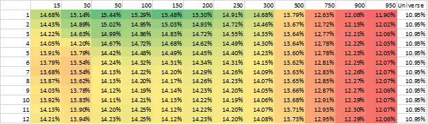
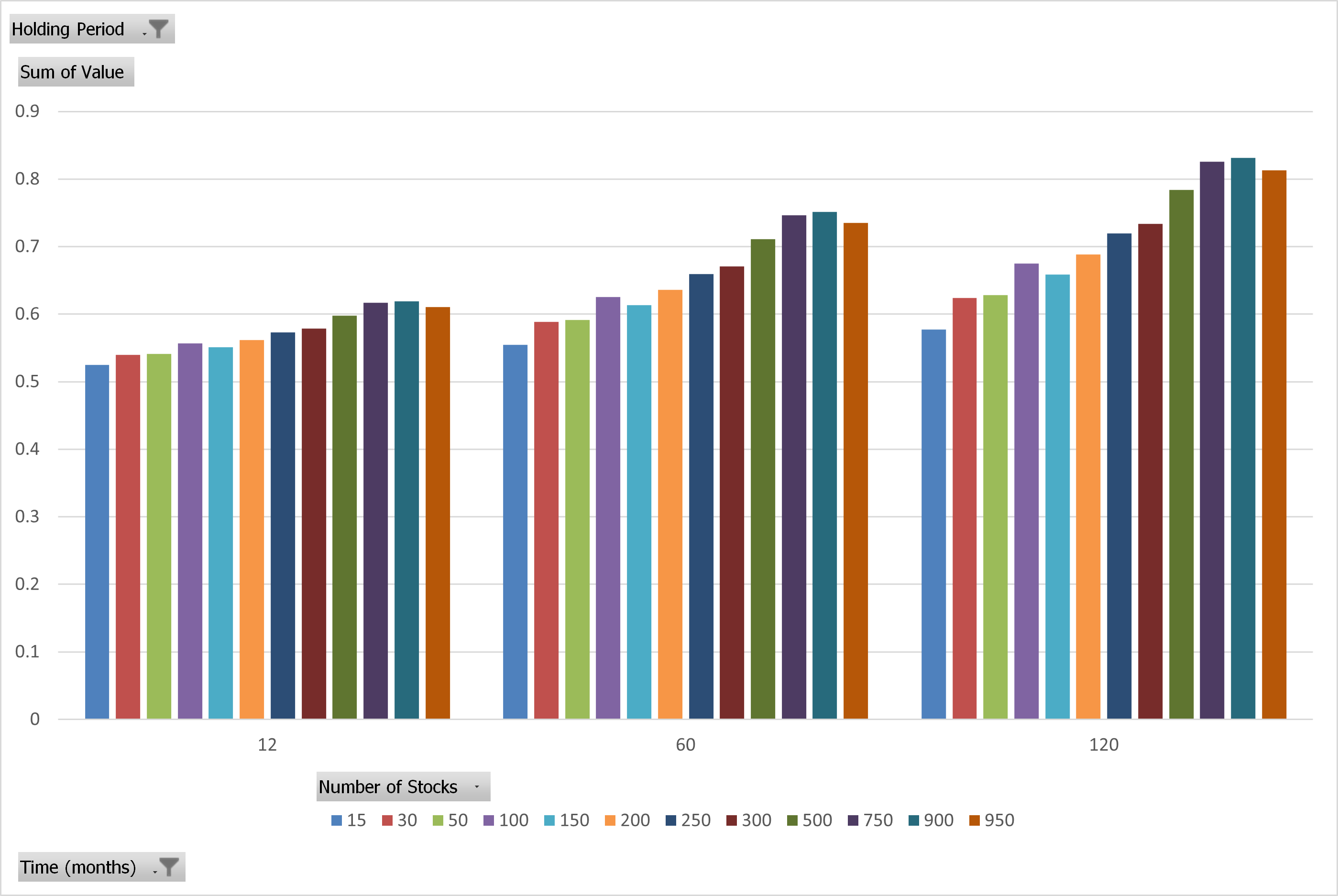
Below are the probabilities to Value portfolios when the rebalance period is 3 months and the portfolio is equal-weighted. The time period we assess the probability of beating the market is either 12 months, 60 months, or 120 months, the same as above.
Value Portfolios’ Probability of Beating the Market
The results are hypothetical results and are NOT an indicator of future results and do NOT represent returns that any investor actually attained. Indexes are unmanaged and do not reflect management or trading fees, and one cannot invest directly in an index.
As we see, the probabilities when going from 50 stocks to 750 stocks are about the same.
This is in direct conflict with the results in section 2 where we assumed means are the same for different factor portfolios.(13)
So what changed in our analysis that made the results so different from the original paper?
We used the historical average returns for each factor portfolio vs assuming they were all the same.
Overall, we do not see a clear relationship between the number of stocks and the probability of beating the market.
Next, we move on to Momentum.
Factor 2: Momentum
To test the Momentum factor, we generate a universe of the 1,000 largest firms from 7/1/1971 through 12/31/2020. Every month, the 1,000 largest firms are chosen. Financials are included for this factor.
Similar to Value, every month, we simply pick the top N names on 12_2 Momentum—the past 12-month’s total return excluding last month. We allow the number of stocks (N) to vary from a 15 stock portfolio up to a 950 stock portfolio on Momentum.
We also allow the rebalance frequency to vary. It can range from 1 month to 12 months. For portfolios held over 1 month, overlapping portfolios are formed.
The portfolios are then either equal-weighted or market-cap weighted. All results shown below are gross of any fees or transaction costs. The results from 7/1/1971 through 12/31/2020 are shown below.
Market-cap weighted CAGR
The results are hypothetical results and are NOT an indicator of future results and do NOT represent returns that any investor actually attained. Indexes are unmanaged and do not reflect management or trading fees, and one cannot invest directly in an index.
Equal-weighted CAGR
The results are hypothetical results and are NOT an indicator of future results and do NOT represent returns that any investor actually attained. Indexes are unmanaged and do not reflect management or trading fees, and one cannot invest directly in an index.
Similar to value, simply adding more and more stocks for Momentum portfolios, does not generate the same mean. A 750-stock momentum portfolio has a mean that is lower than the mean for a 50-stock momentum portfolio.
What about the standard deviation and correlation inputs?
Not surprisingly, a 50-stock, 3-month rebalanced equal-weighted portfolio correlates 0.7876 to the market-cap-weighted universe portfolio with monthly volatility of 7.82%, while a 950-stock, 3-month rebalanced market-cap-weighted portfolio correlates 0.9658 to the market-cap-weighted universe portfolio with monthly volatility of 4.99%. This compares to the universe’s monthly volatility of 4.50%.
So simply examining the 50-stock and 950-stock examples within the model, we have competing inputs, whereby, in a competition between the two portfolios, the 50-stock portfolio is helped by having a higher mean, but is hurt (relatively) by having (1) higher volatility and (2) a lower correlation to the market portfolio it is trying to beat.
What happens if we put all the portfolios into the model—what is the probability of beating the market?
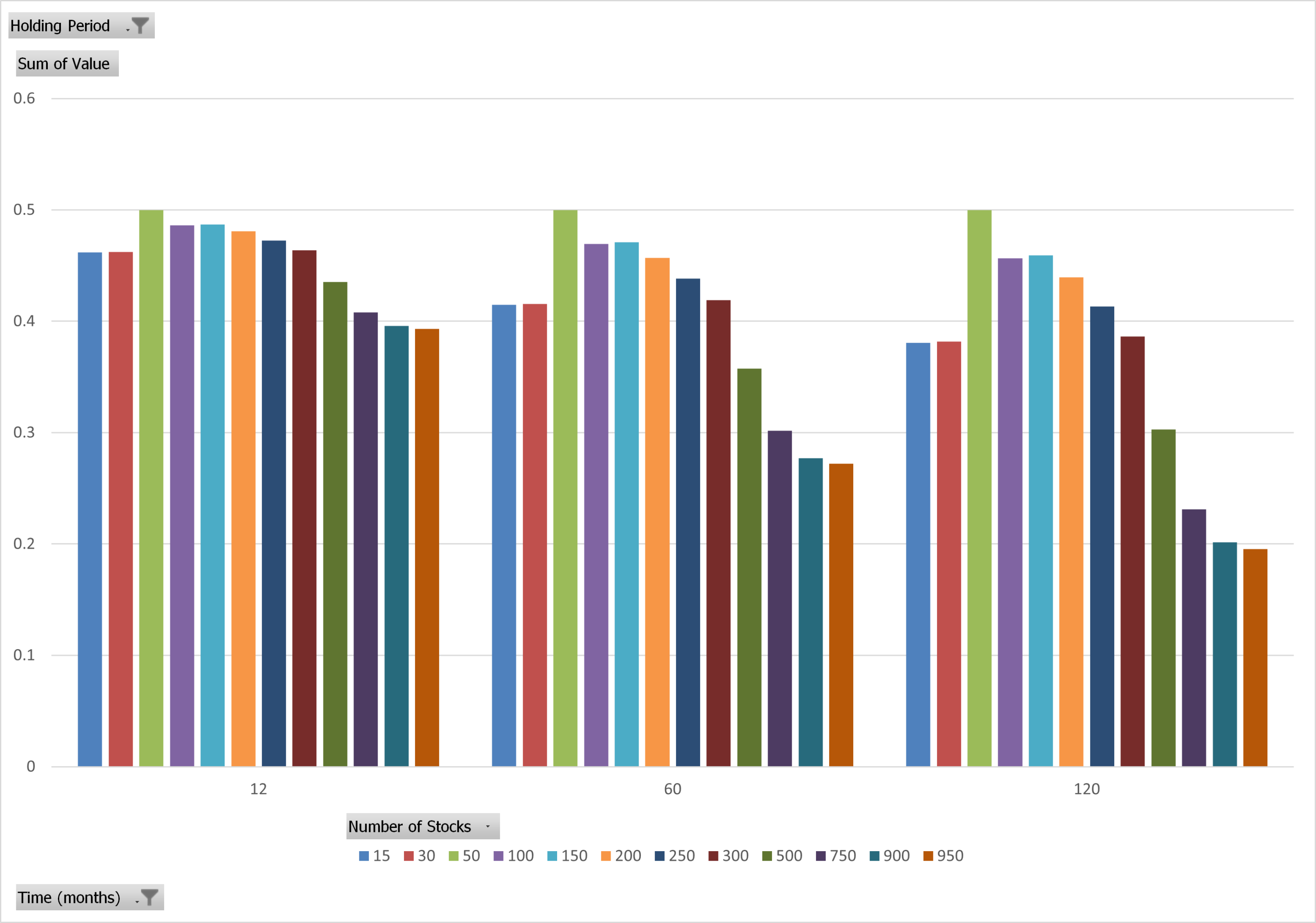
Below are the probabilities for Momentum portfolios when the rebalance period is 3 months, and the portfolio is equal-weighted. The time period we assess the probability of beating the market is either 12 months, 60 months, or 120 months, the same as above.
Momentum Portfolios’ Probability of Beating the Market
The results are hypothetical results and are NOT an indicator of future results and do NOT represent returns that any investor actually attained. Indexes are unmanaged and do not reflect management or trading fees, and one cannot invest directly in an index.
As we see, the probability of beating the market when going from 50 stocks to 750 stocks is about the same—similar to Value. The results are similar for market-cap-weighted portfolios.
Overall, and similar to Value, we do not see a pattern whereby simply adding more stocks substantially and significantly increases the probability of beating the market when examining Momentum portfolios.
Last, we move on to Low Beta.
Factor 3: Low Beta
To test the Beta factor(14) we again generate a universe of the 1,000 largest firms from 7/1/1971 through 12/31/2020. Every month, the 1,000 largest firms are chosen. Financials are included for this factor. Beta is measured using a one-year regression of the daily stock returns against the market stock returns.
Every month, we simply pick the top N names on Low Beta. We allow the number of stocks (N) to vary from a 15 stock portfolio to a 950 stock portfolio formed on Low Beta.
We also allow the rebalance frequency to vary. It can range from 1 month to 12 months. For portfolios held over 1 month, overlapping portfolios are formed.
The portfolios are then either equal-weighted or market-cap weighted. All results shown below are gross of any fees or transaction costs. The results from 7/1/1971 through 12/31/2020 are shown below.
Market-cap weighted CAGR
The results are hypothetical results and are NOT an indicator of future results and do NOT represent returns that any investor actually attained. Indexes are unmanaged and do not reflect management or trading fees, and one cannot invest directly in an index.
Equal-weighted CAGR
The results are hypothetical results and are NOT an indicator of future results and do NOT represent returns that any investor actually attained. Indexes are unmanaged and do not reflect management or trading fees, and one cannot invest directly in an index.
Here, we notice something different than Value and Momentum—adding more stocks does not necessarily hurt the returns!
In contrast to value and momentum factor portfolios, the mean is very similar from 50 stocks through 950 stocks.
Why might this be?
Well, the low beta anomaly reflects the finding that firms with lower beta have higher returns in the future than is expected by the CAPM, and higher beta stocks have lower returns in the future than is predicted by the CAPM.
In other words, the future performance is about the same for all deciles of firms sorted on Beta!
This is shown in the image below looking at returns to the decile sorts on Beta.
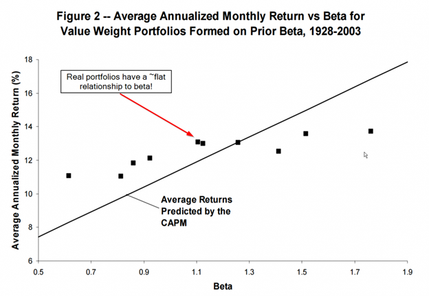
The image above highlights that when sorting firms into deciles on Beta, lower beta firms have similar returns to higher beta firms. The CAPM model would predict a linear relationship; hence, the Beta anomaly.
Thus, for the low beta factor, the mean is going to be very similar as we move from 50 to 950 stock portfolios.
Once again—what about the other inputs to our model?
Not surprisingly, a 50-stock, 3-month rebalanced equal-weighted portfolio correlates 0.6562 to the market-cap-weighted universe portfolio with monthly volatility of 3.64%, while a 950-stock, 3-month rebalanced equal-weighted portfolio correlates 0.9618 to the market-cap-weighted universe portfolio with monthly volatility of 4.90%. This compares to the universe’s monthly volatility of 4.50%.
So within our model to predict the probability of beating the market, the 50-stock portfolio will be helped by having lower monthly volatility but will be hurt by having a lower correlation. The 950-stock portfolio will be hurt by having higher monthly volatility but will be helped by having a higher correlation.
However, different than Value and Momentum—the mean is almost the same!
What happens if we put all the portfolios into the model—what is the probability of beating the market?
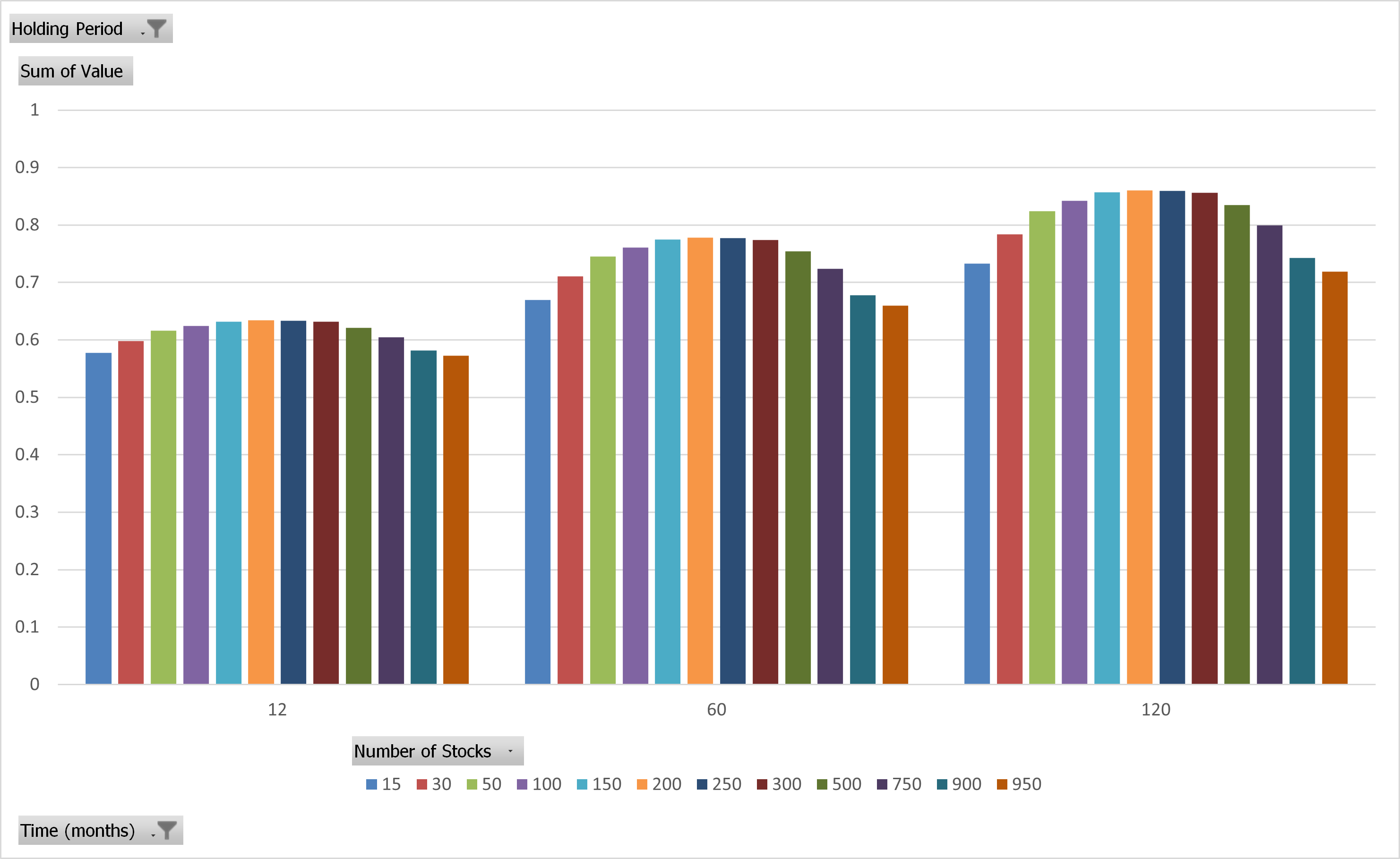
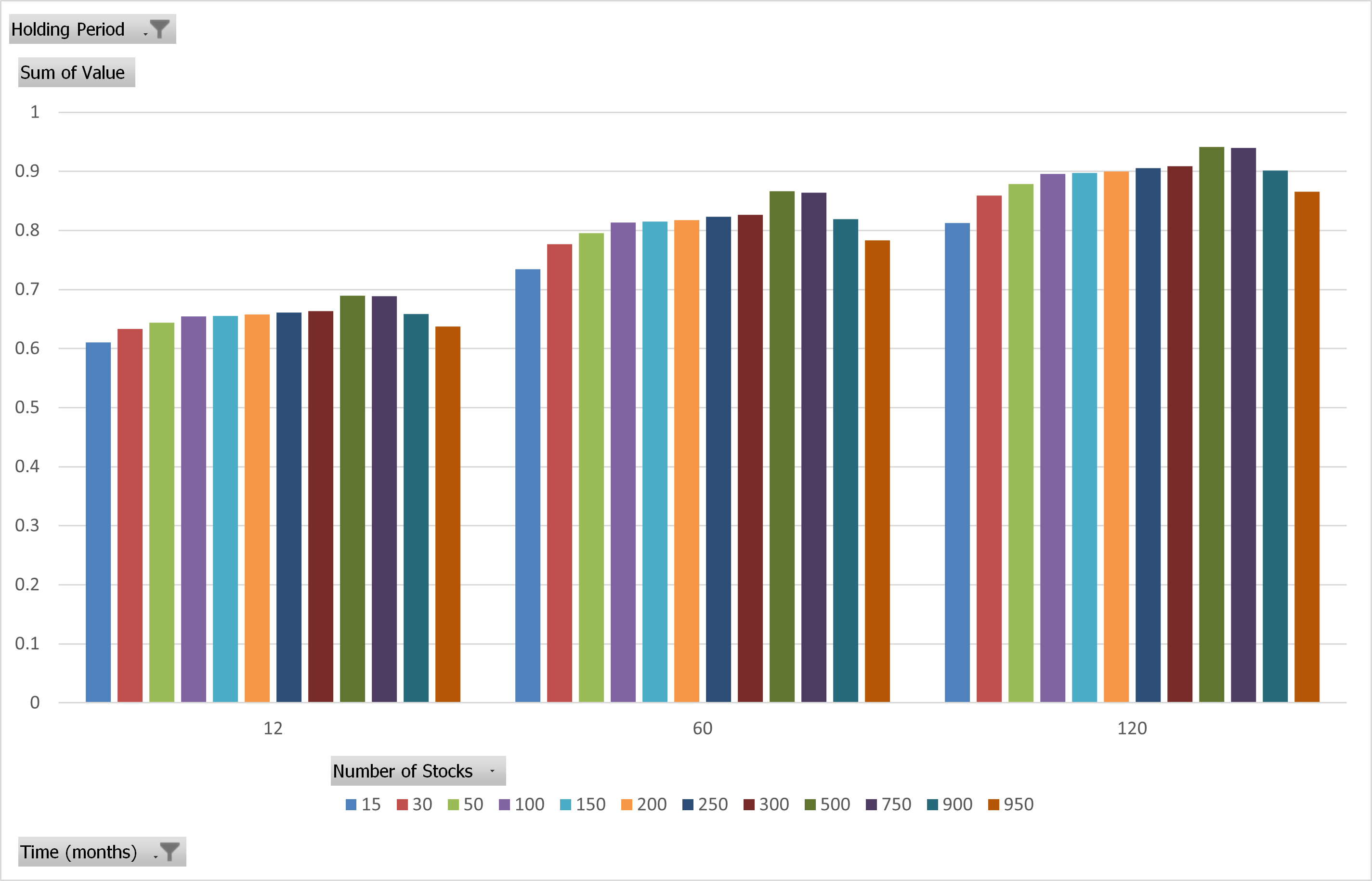
Below are the probabilities to low beta portfolios when the rebalance period is 3 months, and the portfolio is equal-weighted. The time period we assess the probability of beating the market is either 12 months, 60 months, or 120 months, the same as above.
Low Beta Portfolios’ Probability of Beating the Market
The results are hypothetical results and are NOT an indicator of future results and do NOT represent returns that any investor actually attained. Indexes are unmanaged and do not reflect management or trading fees, and one cannot invest directly in an index.
In contrast to value and momentum, here we get a nice linear relationship—add more stocks and you will significantly increase your chances of beating the market. At a 10-year time horizon (120 months), the 50-stock portfolio has a 63% chance of beating the market, while the 750 stock portfolio has an 83% chance. The results are similar for market-cap-weighted portfolios.
Overall, the results for Low Beta are different than for Value and Momentum.
Here’s the takeaway about portfolio construction: if one believes that by simply adding more stocks, the mean return to the portfolio will not change, the model will predict a higher chance of beating the market. For low beta, this seems like a reasonable conclusion. However, for Value and Momentum, adding more and more stocks, at least historically, significantly changed the mean return.
Before we move on, let’s turn back to the Value portfolios, with the probability of beating the market re-shown below.
Value Portfolios’ Probability of Beating the Market

The results are hypothetical results and are NOT an indicator of future results and do NOT represent returns that any investor actually attained. Indexes are unmanaged and do not reflect management or trading fees, and one cannot invest directly in an index.
Some may view this image and ask—well if the ex-ante probability is the same/similar using this model for a 50-stock portfolio, relative to a 250-stock portfolio, why wouldn’t we just use the 250-stock portfolio?
We discuss this in the next section.
Section 4: What Are the Potential Benefits of Portfolio Concentration?
In the last section, we examined three factors—Value, Momentum, and Low Beta. The Value and Momentum factors, where the historical mean varied greatly depending on the number of stocks, did not have a simple significant relationship between portfolio construction and the reliability of outcomes. If anything, the model suggests that significantly diluting (900+ stocks) a value or momentum factor portfolio may decrease your chances of beating the market over the long haul relative to more concentrated portfolios.
However, it is also true that a super-concentrated value or momentum portfolio, with 50 stocks, didn’t increase your odds of beating the market over the long haul versus a 250 stock portfolio.
So why then, do we prefer 50 stock portfolios versus 250 stock portfolios?
On one hand, there are clearly drawbacks of concentrated high active-share portfolios in general: much higher tracking error, which raises short-run career risk concerns, and generally higher volatility. But there is one potential benefit: higher expected returns.
Similar to most decisions in economics, there are no clear “right” answers, there are simply costs and benefits to assess.
Our objective with concentrated portfolios is to provide exposure to high return (and high risk) portfolios that have a high probability of performing over long investment cycles (i.e., 20+ years). One can use the model described above to do a horse race comparison of the probability of a 50-stock factor portfolio beating a diluted factor portfolio (i.e., 250+ stocks). If our objective is long-term outperformance, ideally the model would highlight that we increase our probabilities of winning by owning more concentrated factor portfolios versus diluted portfolios (acknowledging, of course, that these portfolios come with high tracking error and higher volatility).
The portfolio construction model helps us address the question:
What is the probability that a diluted 250-stock value/momentum portfolio beats a concentrated 50 stock value/momentum portfolio?
The future is obviously unknown, but we will use the same historical data to generate the model inputs/outputs.
One edit is needed—we need to assess the correlation of the various Value portfolios against the 50-stock Value portfolio. The same goes for Momentum—we need to assess the correlation of the various Momentum portfolios against the 50-stock momentum portfolio.
In both models, we assume the rebalance frequency is 3 months and the portfolios are equal-weighted.
First, let’s examine Value.
Using the same model, we ask the question—what is the probability that each portfolio (100, 250, 300, etc.) beats the 50-stock equal-weighted portfolio.
The results are shown below.
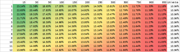
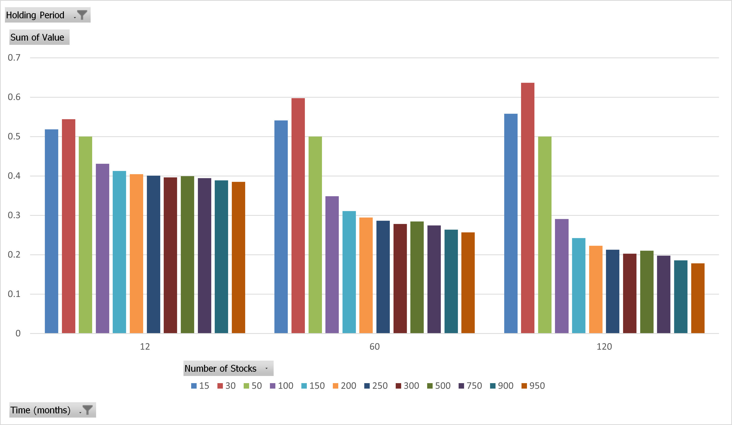
Value Portfolios’ Probability of Beating a 50-Stock Value Portfolio
The results are hypothetical results and are NOT an indicator of future results and do NOT represent returns that any investor actually attained. Indexes are unmanaged and do not reflect management or trading fees, and one cannot invest directly in an index.
The model finds that diluted factor portfolios have a much high probability of underperforming a concentrated portfolio over longer and longer horizons. The more stocks we add, the lower the probability of beating the 50-stock Value portfolio.(15)
We repeat the same process for Momentum and show the results below.
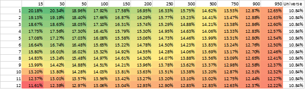
Momentum Portfolios’ Probability of Beating a 50-Stock Momentum Portfolio
The results are hypothetical results and are NOT an indicator of future results and do NOT represent returns that any investor actually attained. Indexes are unmanaged and do not reflect management or trading fees, and one cannot invest directly in an index.
Once again, the model suggests that adding more stocks decreases the probability of beating the 50-stock portfolio.
One also notices that 15 and 30 stock portfolios slightly beat the 50-stock model, so in theory, you may consider running really concentrated momentum portfolios. However, we’d note that the probability is still near 50%-60% over 1-year, 5-year, and 10-year time horizons, and we’d also point out that the risk/return profile on a 50-stock momentum strategy is already pushing the limits of what most investors can handle.
Thus, the main takeaway is the following—for Value and Momentum, the model suggests that adding more stocks to a factor portfolio actually decreases the probability of beating a 50-stock value or momentum factor portfolio. This result is entirely driven by the fact that more concentrated factor portfolios have historically delivered more factor exposure, and thus more expected returns (and risk).
The Global Benefits of Concentrated Factor Portfolios
Of course, there are other potential benefits associated with more concentrated value and momentum factor portfolios.
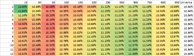
Let’s examine the historical mean return (gross) of various factor portfolios. Below is the data for the CAGR (compounded annualized growth rate) while varying the portfolio N’s, keeping the rebalance frequency to 3-months, and equal-weighting the portfolios—while this was shown above, we highlight the results below:
Momentum:

The results are hypothetical results and are NOT an indicator of future results and do NOT represent returns that any investor actually attained. Indexes are unmanaged and do not reflect management or trading fees, and one cannot invest directly in an index.
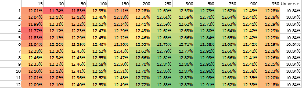
Value:

The results are hypothetical results and are NOT an indicator of future results and do NOT represent returns that any investor actually attained. Indexes are unmanaged and do not reflect management or trading fees, and one cannot invest directly in an index.
More concentrated portfolios have historically delivered higher expected returns for Value and Momentum. We believe this is due to the fact that these portfolios, by construction, are more concentrated in the factor exposure. If one believes that factor exposures proxy for various market risk/pain, we would expect this outcome historically, and we would expect this in the future.
Second, we can examine the correlations. Below are the correlations against the market-cap-weighted universe portfolio.
Momentum:

The results are hypothetical results and are NOT an indicator of future results and do NOT represent returns that any investor actually attained. Indexes are unmanaged and do not reflect management or trading fees, and one cannot invest directly in an index.
Value:

The results are hypothetical results and are NOT an indicator of future results and do NOT represent returns that any investor actually attained. Indexes are unmanaged and do not reflect management or trading fees, and one cannot invest directly in an index.
As we see, by adding more stocks, we are generating a higher correlation to the market portfolio. Going back to portfolio theory, even if the returns to the 50-stock and the 250-stock portfolio were exactly the same (they are not), one may prefer a 50-stock factor portfolio because of the lower correlation to the existing portfolio (which is likely concentrated in market beta).
Thus, more concentrated portfolios can actually enhance overall portfolio diversification.
Finally, we examine the active share of the factor portfolios. While not necessarily indicative of future returns, active share highlights how different a portfolio is relative to the market portfolio.(16) Given the fact that market exposure is essentially free, one would prefer (all else being equal) to pay higher fees for active management if the active management is providing a different portfolio with unique benefits to the overall portfolio.
Below we show the active share to the portfolios relative to the market-cap-weighted universe portfolio, as of 12/31/2020.
Momentum:

The results are hypothetical results and are NOT an indicator of future results and do NOT represent returns that any investor actually attained. Indexes are unmanaged and do not reflect management or trading fees, and one cannot invest directly in an index.
Value:

The results are hypothetical results and are NOT an indicator of future results and do NOT represent returns that any investor actually attained. Indexes are unmanaged and do not reflect management or trading fees, and one cannot invest directly in an index.
As we see above, and not surprisingly, portfolios with fewer stocks have a higher active share.
Taken together, we prefer the benefits of more concentrated factor portfolios relative to diluted factor portfolios.
Of course, concentrated factor portfolios are not a panacea. With more ‘pure’ factor exposure comes the potential for more volatility and a higher chance of being very different than the generic market–both the good and bad times. These elements of concentration can cause behavioral issues for investors more focused on short-term relative performance versus long-term overall portfolio performance.
Conclusions on Portfolio Construction
We started this portfolio construction study by examining a model that predicts the probability of a portfolio beating the market. Using this simple model, we found that small caps have a 50/50 chance to beat large caps. Next, we turned to variations of value portfolios and found that if the mean is the same, simply adding more stocks does increase the probability of beating the market.
However, we then asked the question—should we assume that factor portfolios have similar means? Clearly, this was not the case for the value and momentum factors. After relaxing this assumption, the model finds that the ex-ante probability of value and momentum factor portfolios beating the market does not significantly increase by simply adding more stocks to these portfolios.
Next, we looked at the potential benefits of concentrated factor portfolios. We test various factor portfolios against the 50-stock, equal-weight, 3-month rebalance Value or Momentum portfolios. The model suggests that adding more stocks decreases the probability of beating the 50-stock portfolio. Also, we highlight some additional benefits of more concentrated models—lower correlation to the market portfolio, and thus the potential for stronger diversification benefits for a global multi-asset portfolio. Of course, one can also combine Value and Momentum in a portfolio!
We end our portfolio construction analysis with this note–the reality is that factor concentration comes with costs and benefits.
More concentrated portfolios deliver more impactful doses of the factor–both the good and the bad–whereas more diluted factor portfolios deliver a more market-like return. This statement is intuitive to most, but not for everyone. We hope this portfolio construction piece helps clarify the topic.
Analysis using Ken French Data:
We try to be as open and transparent as possible, and to the best of our abilities, highlight the pros and cons of any approach. In order to facilitate this goal, we will share the underlying file to allow interested readers to generate the images in sections 1 and 2, so readers may verify our results for themselves and check the formulas. Please fill out the form at the end of this section if you are interested in receiving the excel file.
Additionally, in sections 3 and 4, we use time-series return data that we have generated internally. While we trust the numbers, we also wanted to run the analysis using another third-party data resource that is publicly available. So we chose Ken French’s Data Library to examine Value (formed on P/E) and Momentum portfolios. We wanted to see if we generated the same results. These calculations are also in the excel file.
Ken French Data Used:
- The Market Return
- The Value Portfolios, formed on P/E
- The Momentum Portfolios, formed on 12_2 Momentum
You’ll notice within the excel file, that we had to add the Risk-Free rate back to the Market minus risk-free (Mkt-RF) returns in order to get the market return. Also, you will see that the Value Portfolios run from July of 1951 through December of 2020, while the Momentum portfolios run from January of 1927 through December of 2020.
Using the Ken French Data for Value and Momentum, we create the top 10%, top 20%, top 30% and top 50% portfolios as follows:
- Top 10% — simply the top Decile on Value or Momentum
- Top 20% — an average of the top two (2) deciles on Value or Momentum
- Top 30% — an average of the top three (3) deciles on Value or Momentum
- Top 50% — an average of the top five (5) deciles on Value or Momentum
This was done as the Momentum portfolios only have decile splits, while the data on the P/E portfolios does include the top 20% and 30%. However, for consistency, we just average the top N deciles for Value and Momentum.(17)
Back to the original question–Does adding more stocks substantially increase the probability of beating the market?
No.
And for our second question–Does adding more stocks substantially increase the probability of beating more concentrated factor portfolios?
No.
Below are the results for Value.
Section 3 Results–What is the probability of beating the market?
Value Portfolios (Equal-weighted) Probability of Beating the Market:
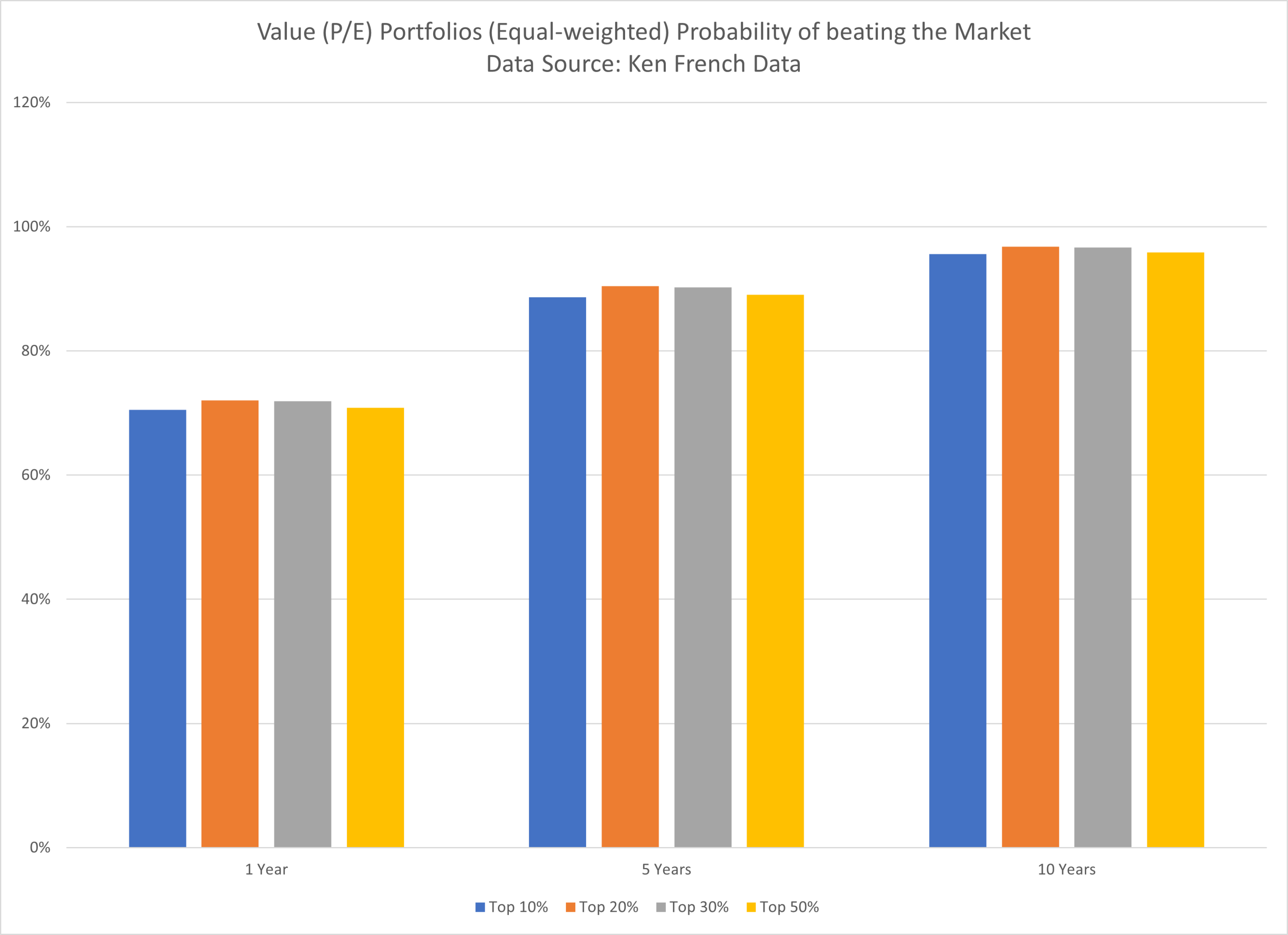
The results are hypothetical results and are NOT an indicator of future results and do NOT represent returns that any investor actually attained. Indexes are unmanaged and do not reflect management or trading fees, and one cannot invest directly in an index.
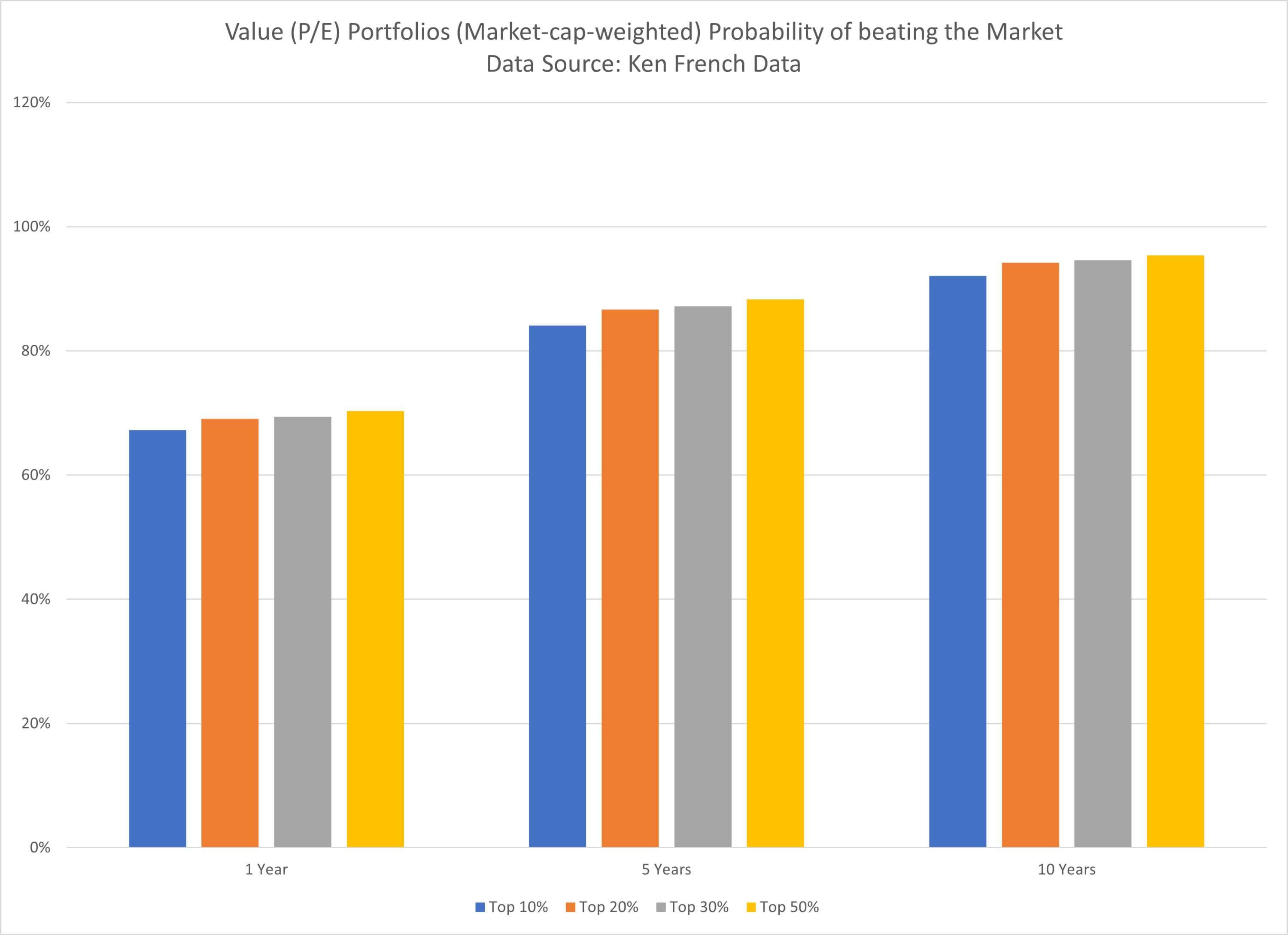
Value Portfolios (Market-cap-weighted) Probability of Beating the Market:
The results are hypothetical results and are NOT an indicator of future results and do NOT represent returns that any investor actually attained. Indexes are unmanaged and do not reflect management or trading fees, and one cannot invest directly in an index.
As shown above, adding more stocks does not substantially increase the reliability, i.e. the probability of beating the market using the proposed model.
So what about beating the top decile on Value with more diluted value factor portfolios?
Section 4 Results–What is the probability of beating the top decile on Value?
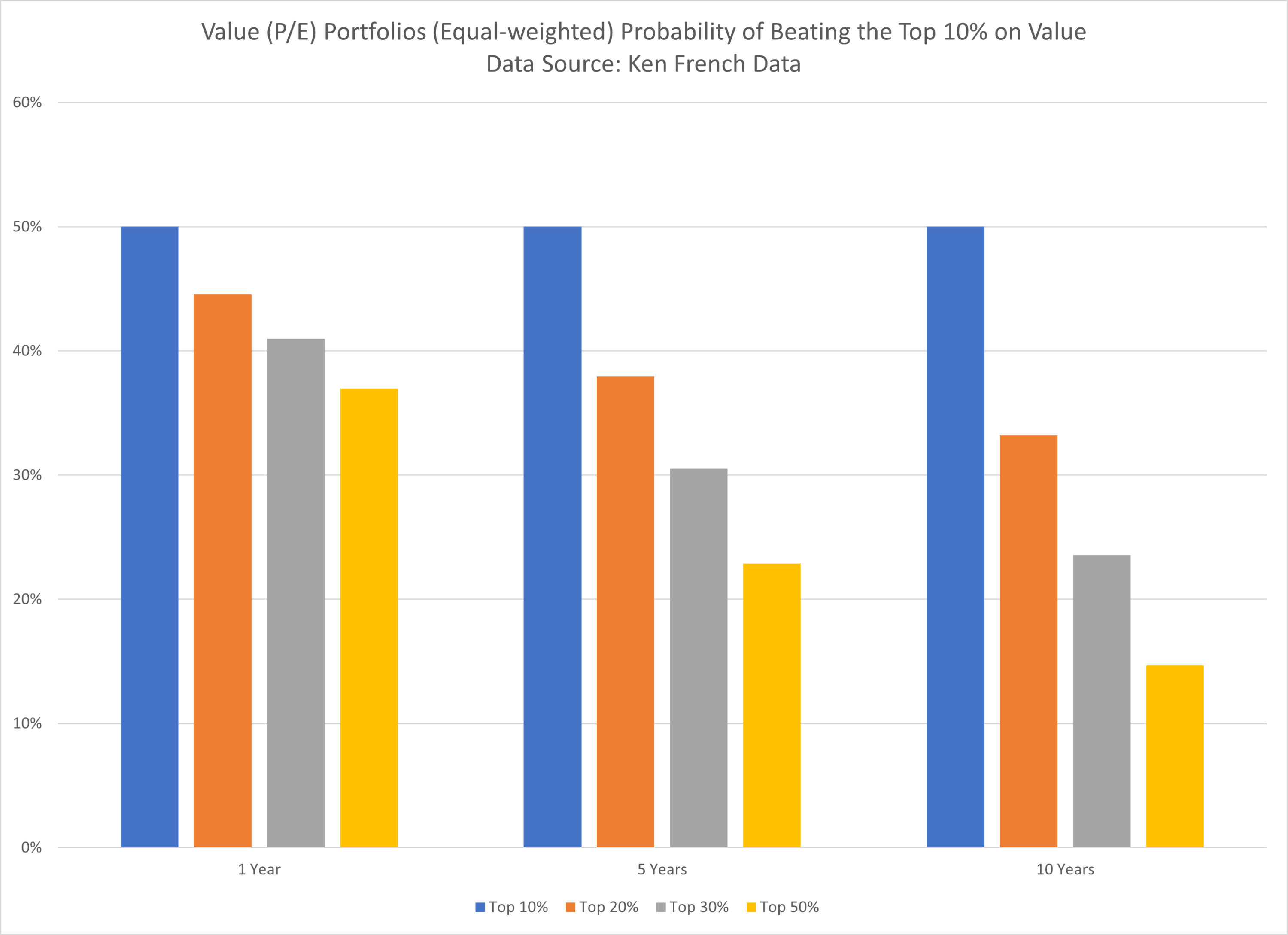
Equal-weighted Probability of Beating the Top Decile on Value:
The results are hypothetical results and are NOT an indicator of future results and do NOT represent returns that any investor actually attained. Indexes are unmanaged and do not reflect management or trading fees, and one cannot invest directly in an index.
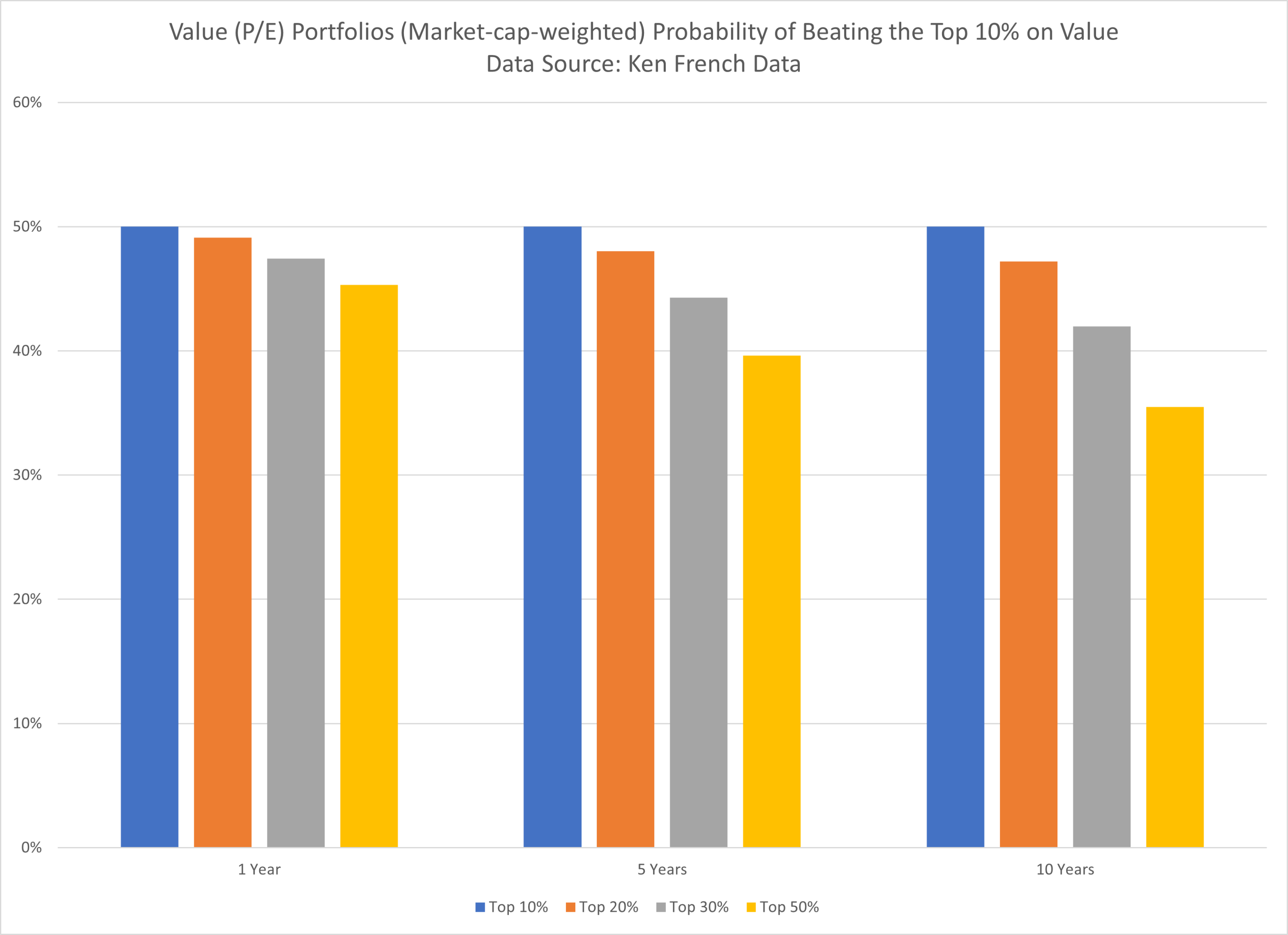
Market-cap-weighted Probability of Beating the Top Decile on Value:
The results are hypothetical results and are NOT an indicator of future results and do NOT represent returns that any investor actually attained. Indexes are unmanaged and do not reflect management or trading fees, and one cannot invest directly in an index.
Once again we find the same result as in our analysis using our data–concentrated factor portfolios reliably beat more diversified factor portfolios.
Now we turn to Momentum using Ken French’s Data.
Section 3 Results–What is the probability of beating the market?
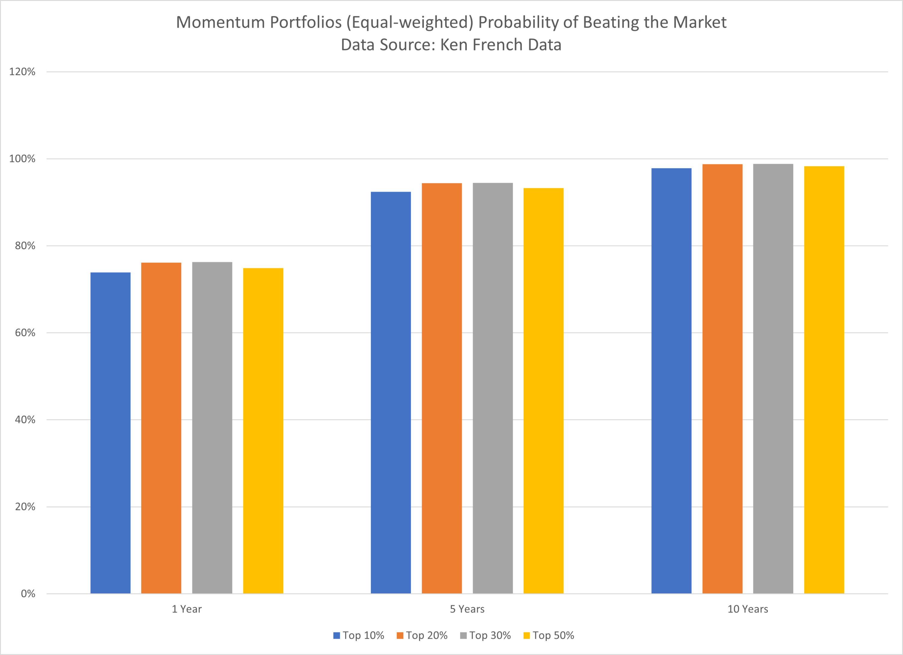
Momentum Portfolios (Equal-weighted) Probability of Beating the Market:
The results are hypothetical results and are NOT an indicator of future results and do NOT represent returns that any investor actually attained. Indexes are unmanaged and do not reflect management or trading fees, and one cannot invest directly in an index.
Momentum Portfolios (Market-cap-weighted) Probability of Beating the Market:

The results are hypothetical results and are NOT an indicator of future results and do NOT represent returns that any investor actually attained. Indexes are unmanaged and do not reflect management or trading fees, and one cannot invest directly in an index.
As shown above, adding more stocks does not substantially increase the reliability, i.e. the probability of beating the market using the proposed model.
So what about beating the top decile on Momentum?
Section 4 Results–What is the probability of beating the top decile on Momentum?
Equal-weighted Probability of Beating the Top Decile on Momentum:
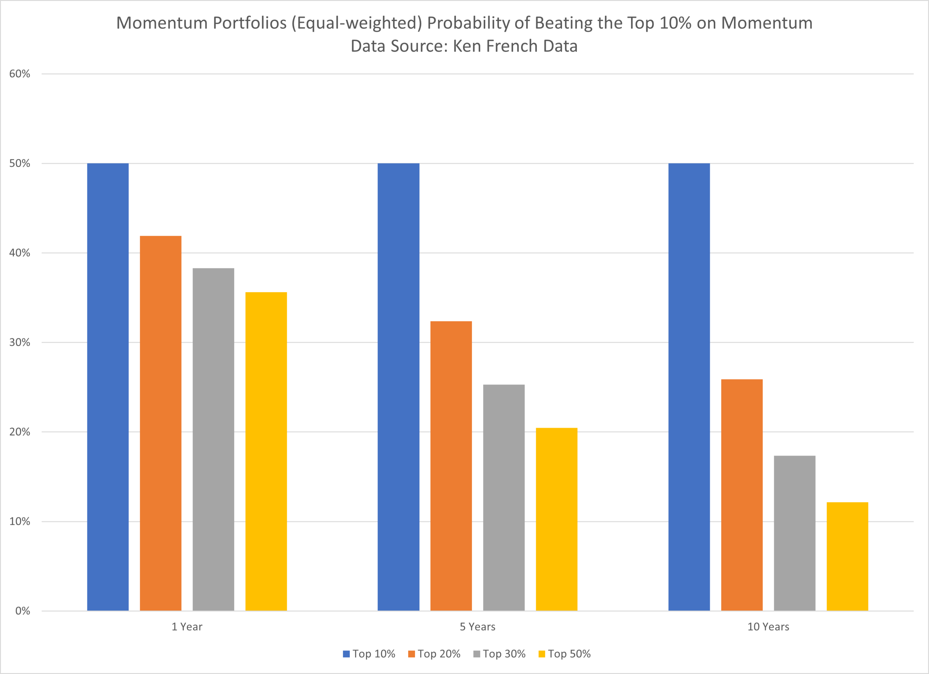
The results are hypothetical results and are NOT an indicator of future results and do NOT represent returns that any investor actually attained. Indexes are unmanaged and do not reflect management or trading fees, and one cannot invest directly in an index.
Market-cap-weighted Probability of Beating the Top Decile on Momentum:
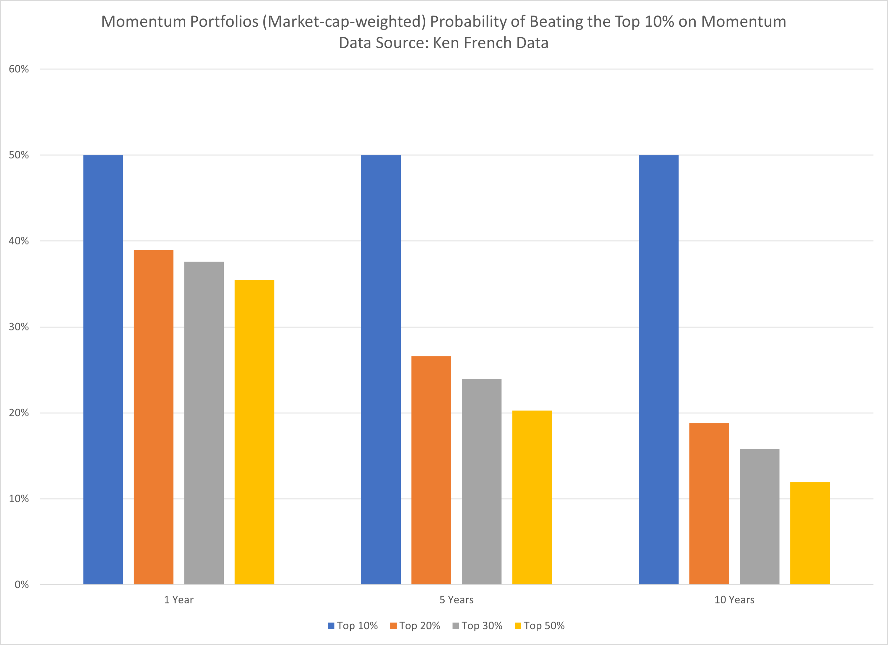
The results are hypothetical results and are NOT an indicator of future results and do NOT represent returns that any investor actually attained. Indexes are unmanaged and do not reflect management or trading fees, and one cannot invest directly in an index.
Once again we find the same result as in our analysis using our data–concentrated portfolios reliably beat their more diversified counterparts.
Regardless of whether we use our own factor data or Ken French’s factor data, the results don’t change:
- Concentrated value and momentum factor portfolios reliably beat the diluted value and momentum factor portfolios over time.
Of course, none of this analysis is meant to predict the future since the model used for long-term returns is simple and past performance does not necessarily imply future performance.
Looking for the underlying spreadsheet and data? Shoot us a note.
References[+]
| ↑1 | Please note that in the context of long/short factor investing, which is more focused on Sharpe optimization and the use of leverage, the discussion is more nuanced. If you are interested in this topic we recommend starting with research from authors associated with AQR. |
|---|---|
| ↑2 | For other factors, i.e., those more focused on risk-mitigation versus high expected returns, this may not be the case. |
| ↑3 | This would be like Steve Kerr telling Steph Curry, the best 3-point shooter in the history of the NBA, that Steph really needs to cut back on his 3-point shots. |
| ↑4 | Of course, models are only approximations of reality, and models can be highly driven by assumptions. |
| ↑5 | Note, this assumption was confirmed by representatives at DFA, but this isn’t clearly stated in the paper; however, this assumption is implied because the simulations used in the study are constructed to have similar factor profiles, which essentially implies an assumption of equal returns. See this article highlighting that characteristics drive stock returns. |
| ↑6 |
 |
| ↑7 | Of note, this normally entails holding fewer small-cap stocks. |
| ↑8 | This is based on prior research on this topic that portfolios with similar characteristics profiles should deliver similar expected returns. Communications with the authors confirm that assuming equal returns is appropriate. |
| ↑9 | Using historical data, is the best we can do. |
| ↑10 | similar to most academic studies on Value |
| ↑11 | Throughout the analysis we look at total returns which include distributions such as dividends. All results are gross of any transaction costs. |
| ↑12 | Hence, Value is a “factor”. |
| ↑13 | Given that this factor is Value, the results are similar if we change the rebalance period to 12 months, and either equal-weighted or value-weight the portfolio. |
| ↑14 | Defined here as investing in Lower Beta stocks, without using leverage. |
| ↑15 | We notice that the 50-stock portfolio is 50%, which highlights that if the mean of the lognormal is 0, one gets a 50/50 chance to win/lose. |
| ↑16 | See this article by Larry |
| ↑17 | Note–if we use the top 20% and 30% directly on Value, the results are similar. We examine the equal-weight and value-weight (i.e. market-cap-weight) portfolios. Yes, I know that (1) taking the arithmetic average of the top five market-cap-weighted deciles is not the same as (2) picking the top 50% of stocks on P/E or Momentum, and then market-cap-weighting. But, in order to use a publicly available data source, this is the best I can do. |
About the Author: Jack Vogel, PhD
—
Important Disclosures
For informational and educational purposes only and should not be construed as specific investment, accounting, legal, or tax advice. Certain information is deemed to be reliable, but its accuracy and completeness cannot be guaranteed. Third party information may become outdated or otherwise superseded without notice. Neither the Securities and Exchange Commission (SEC) nor any other federal or state agency has approved, determined the accuracy, or confirmed the adequacy of this article.
The views and opinions expressed herein are those of the author and do not necessarily reflect the views of Alpha Architect, its affiliates or its employees. Our full disclosures are available here. Definitions of common statistics used in our analysis are available here (towards the bottom).
Join thousands of other readers and subscribe to our blog.